On a conjecture of Goppa on codes and counting points hyperelliptic curves

What is the best code of a given length? This natural, but very hard, question motivates the following definition.

Definition: Let $B_q(n,d)$ denote the largest $k$ such that there exists a [ $n,k,d$ ]-code in $GF(q)^n$ .

Determining $B_q(n,d)$ is one of the main problems in the theory of error-correcting codes.

Let $C_i$ be a sequence of linear codes with parameters [ $n_i,k_i,d_i$ ] such that $n_i\rightarrow \infty$ as $i \to \infty$ , and such that both the limits $R=\lim_{i\to \infty}\frac{k_i}{n_i}$ and $\delta=\lim_{i\rightarrow \infty}\frac{d_i}{n_i}$ exist. The Singleton (upper) bound implies $R+\delta\leq 1$ .

Let $\Sigma_q$ denote the set of all $(\delta,R)\in [0,1]^2$ such that there exists a sequence $C_i$ , $i=1,2,...$ , of [ $n_i,k_i,d_i$ ]-codes for which $\lim_{i\to \infty} d_i/n_1=\delta$ and $\lim_{i\rightarrow \infty} k_i/n_i=R$ .

Theorem (Manin [SS]): There exists a continuous decreasing function $\alpha_q:[0,1]\to [0,1]$ , such that

$\alpha_q$ is strictly decreasing on [ $0,\frac{q-1}{q}$ ],
$\alpha_q(0)=1$ ,
if ${\frac{q-1}{q}}\leq x\leq 1$ then $\alpha_q(x)=0$ ,
$\Sigma_q=\{(\delta,R)\in [0,1]^2\ |\ 0\leq R\leq \alpha_q(\delta)\}$ .

Theorem (Gilbert-Varshamov): We have $\alpha_q(x)\geq 1- x\log_q(q-1)-x\log_q(x)-(1-x)\log_q(1-x)$ . In other words, for each fixed $\epsilon >0$ , there exists an [ $n,k,d$ ]-code $C$ (which may depend on $\epsilon$ ) with $R(C)+\delta(C)\geq 1- \delta(C)\log_q({\frac{q-1}{q}})-\delta(C)\log_q(\delta(C))-(1-\delta(C))\log_q(1-\delta(C))-\epsilon$ . In particular, in the case $q=2$ , $\alpha_q(x)\geq1-H_2(\delta)$ , where $H_q(\delta)=\delta\cdot \log_q(q-1)-\delta\log_q(\delta)-(1-\delta)\log_q(1-\delta)$ is the entropy function (for a q-ary channel).

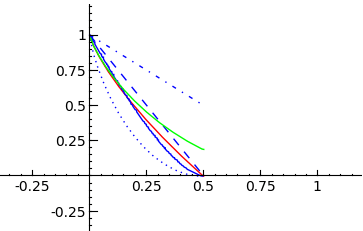
Plot of the Gilbert-Varshamov (dotted), Elias (red), Plotkin (dashed), Singleton (dash-dotted), Hamming (green), and MRRW (stepped) curves using SAGE:

Not a single value of $\alpha_q(x)$ is known for $0<x<{\frac{q-1}{q}}$ !

Goppa’s conjecture: $\alpha_q(x) = 1-H_2(\delta)$ . (In other words, the Gilbert-Varshamov lower bound is actually attained in the case $q=2$ .)

Though my guess is that Goppa’s conjecture is true, it is known (thanks to work of Zink, Vladut and Varshamov) that the q-ary analog of Goppa’s conjecture is false for $q>49$ . On the other hand, we have the following theorem [J].

Theorem: If $B(1.77,p)$ is true for infinitely many primes p with $p\equiv 1\pmod 4$ then Goppa’s conjecture is false.

The rest of this post will be devoted to explaining the notation in this Theorem. The notation $B(c,p)$ means: “For all subsets $S\subset GF(p)$ , $|X_S(GF(p))| \leq c\cdot p$ holds.” The notation $X_S$ means: For each non-empty subset $S\subset GF(p)$ , define the hyperelliptic curve $X_S$ by $y^2=f_S(x)$ , where $f_S(x) = \prod_{a\in S}(x-a)$ .

It may seem strange that a statement about the asymptotic bounds of error-correcting curves is related to the number of points on hyperelliptic curves, but for details see [J]. Unfortunately, it appears much more needs to be known about hyperelliptic curves over finite fields if one is to try to use this connection to prove or disprove Goppa’s conjecture.

References:
[J] D. Joyner, On quadratic residue codes and hyperelliptic curves. Discrete Mathematics & Theoretical Computer Science, Vol 10, No 1 (2008).
[SS] S. Shokranian and M.A. Shokrollahi, Coding theory and bilinear complexity, Scientific Series of the International Bureau, KFA Julich Vol. 21, 1994.

Here’s how the above plot is constructed using SAGE:

sage: f1 = lambda x: gv_bound_asymp(x,2) sage: P1 = plot(f1,0,1/2,linestyle=":") sage: f2 = lambda x: plotkin_bound_asymp(x,2) sage: P2 = plot(f2,0,1/2,linestyle="--") sage: f3 = lambda x: elias_bound_asymp(x,2) sage: P3 = plot(f3,0,1/2,rgbcolor=(1,0,0)) sage: f4 = lambda x: singleton_bound_asymp(x,2) sage: P4 = plot(f4,0,1/2,linestyle="-.") sage: f5 = lambda x: mrrw1_bound_asymp(x,2) sage: P5 = plot(f5,0,1/2,linestyle="steps") sage: f6 = lambda x: hamming_bound_asymp(x,2) sage: P6 = plot(f6,0,1/2,rgbcolor=(0,1,0)) sage: show(P1+P2+P3+P4+P5+P6)

If you are interested in computing what c might be in the above statement B(c,p), the following SAGE code may help.
First, the Python function below will return a random list of elements without repetition, if desired) from an object.

def random_elements(F,n,allow_repetition=True):
    """
    F is a SAGE object for which random_element is a method 
    and having >n elements. For example, a finite field. Here 
    n>1 is an integer. The output is to have no repetitions 
    if allow_repetion=False.
    EXAMPLES:
        sage: p = nth_prime(100)
        sage: K = GF(p)
        sage: random_elements(K,2,allow_repetition=False)
        [336, 186]
    The command random_elements(K,p+1,allow_repetition=False)
    triggers a ValueError.
    """
    if (n>F.order()-2 and allow_repetition==False):
        raise ValueError("Parameters are not well-choosen.")
    L = []
    while len(L)<n:
        c = F.random_element()
        if allow_repetition==False:
            if not(c in L):
                L = L+[c]
        else:
            L = L+[c]
    return L

Next, the SAGE code computes $|X_S(GF(p))|/p$ for a particular choice of the parameters. This gives a lower bound for c.

sage: p = nth_prime(100) sage: K = GF(p) sage: R. = PolynomialRing(K, "x") sage: S = random_elements(K,ZZ((p+1)/2),allow_repetition=False) sage: fS = prod([x - a for a in S]) sage: XS = HyperellipticCurve(fS) sage: RR(len(XS.points())/p) 0.975970425138632
Based on experiments with this code, it appears that for “random” chices of S, and p “large”, the quotient $|X_S(GF(p))|/p$ is very close to 1.

M	T	W	T	F	S	S
	1	2	3	4	5	6
7	8	9	10	11	12	13
14	15	16	17	18	19	20
21	22	23	24	25	26	27
28	29	30

Yet Another Mathblog

On a conjecture of Goppa on codes and counting points hyperelliptic curves

Leave a Reply Cancel reply

Yet Another Mathblog

Share this:

Like this:

Related

Leave a Reply Cancel reply