This is an exposition of some ideas of Conway, Curtis, and Ryba on  and a card game called mathematical blackjack (which has almost no relation with the usual Blackjack).
Many thanks to Alex Ryba and Andrew Buchanan for helpful discussions on this post.
Definitions
An m-(sub)set is a (sub)set with m elements. For integers  , a Steiner system S(k,m,n) is an n-set X and a set S of m-subsets having the property that any k-subset of X is contained in exactly one m-set in S. For example, if
  , a Steiner system S(5,6,12) is a set of 6-sets, called hexads, with the property that any set of 5 elements of X is contained in (“can be completed to”) exactly one hexad.
Rob Beezer has a nice Sagemath description of S(5,6,12).
If S is a Steiner system of type (5,6,12) in a 12-set X then any element the symmetric group  of X sends S to another Steiner system
  of X. It is known that if S and S’ are any two Steiner systems of type (5,6,12) in X then there is a
  such that
  . In other words, a Steiner system of this type is unique up to relabelings. (This also implies that if one defines
  to be the stabilizer of a fixed Steiner system of type (5,6,12) in X then any two such stabilizer groups, for different Steiner systems in X, must be conjugate in
  . In particular, such a definition is well-defined up to isomorphism.)
Curtis’ kitten

NICOLE SHENTING – Cats Playing Poker Cards
J. Conway and R. Curtis [Cu1] found a relatively simple and elegant way to construct hexads in a particular Steiner system using the arithmetical geometry of the projective line over the finite field with 11 elements. This section describes this.
Let  denote the projective line over the finite field
  with 11 elements. Let
  denote the quadratic residues with 0, and let
  where
where  and
and  . Let
. Let 
Lemma 1:  is a Steiner system of type
  .
.
The elements of S are known as hexads (in the “modulo 11 labeling”).
 6
2 10
5 7 3
6 9 4 6
2 10 8 2 10
0 1
 	 	 	 	 	6

 	 	 	 	2	 	10

 	 	 	5	 	7	 	3

 	 	6	 	9	 	4	 	6

 	2	 	10	 	8	 	2	 	10

0	 	 	 	 	 	 	 	 	 	1
Curtis’ Kitten.
In any case, the “views” from each of the three “points at infinity” is given in the following tables.
6	10	3
2	7	4
5	9	8
picture at

5	7	3
6	9	4
2	10	8
picture at

5	7	3
9	4	6
8	2	10
picture at
5 7 3
9 4 6
8 2 10
picture at 
Each of these  arrays may be regarded as the plane
  . The lines of this plane are described by one of the following patterns.


 slope 0
slope infinity
slope -1
slope 1
slope 0


slope infinity


slope -1


slope 1
The union of any two perpendicular lines is called a cross. There are 18 crosses. The complement of a cross in is called a square. Of course there are also 18 squares. The hexads are
 ,
,- the union of any two (distinct) parallel lines in the same picture,
- one “point at infinity” union a cross in the corresponding picture,
- two “points at infinity” union a square in the picture corresponding to the omitted point at infinity.
Lemma 2 (Curtis [Cu1]) There are 132 such hexads (12 of type 1, 12 of type 2, 54 of type 3, and 54 of type 4). They form a Steiner system of type $(5,6,12)$.
The MINIMOG description
Following Curtis’ description [Cu2] of a Steiner system  using a $4\times 6$ array, called the MOG, Conway [Co1] found and analogous description of using a
  array, called the MINIMOG. This section is devoted to the MINIMOG. The tetracode words are
0	0	0	0		0	+	+	+		0	-	-	-
+	0	+	-		+	+	-	0		+	-	0	+
-	0	-	+		-	+	0	-		-	-	+	0
With ”0″=0, “+”=1, “-“=2, these vectors form a linear code over GF(3). (This notation is Conway’s. One must remember here that “+”+”+”=”-“!) They may also be described as the set of all 4-tuples in of the form
 

where abc is any cyclic permutation of 012. The MINIMOG in the shuffle numbering is the array

We label the rows of the MINIMOG array as follows:
- the first row has label 0,
- the second row has label +,
- the third row has label –
A col (or column) is a placement of three + signs in a column of the MINIMOG array. A tet (or tetrad) is a placement of 4 + signs having entries corresponding (as explained below) to a tetracode.
+	+	+	+


0	0	0	0
+
 	+	+	+

0	+	+	+
+

 	+	+	+


0	-	-	-
 	+
+	 	+
 	 	 	+

+	0	+	-
 	 	 	+
+	+
 	 	+

+	+	-	0
 	 	+
+	 	 	+
 	+


+	-	0	+
 	+
 	 	 	+
+	 	+

-	0	-	+
 	 	+
 	+
+	 	 	+

-	+	0	-
 	 	 	+
 	 	+
+	+


-	-	+	0
Each line in with finite slope occurs once in the part of some tet. The odd man out for a column is the label of the row corresponding to the non-zero digit in that column; if the column has no non-zero digit then the odd man out is a “?”. Thus the tetracode words associated in this way to these patterns are the odd men out for the tets. The signed hexads are the combinations $6$-sets obtained from the MINIMOG from patterns of the form
col-col, col+tet, tet-tet, col+col-tet.
Lemma 3 (Conway, [CS1], chapter 11, page 321) If we ignore signs, then from these signed hexads we get the 132 hexads of a Steiner system . These are all possible $6$-sets in the shuffle labeling for which the odd men out form a part (in the sense that an odd man out “?” is ignored, or regarded as a “wild-card”) of a tetracode word and the column distribution is not  in any order.
Furthermore, it is known [Co1] that the Steiner system in the shuffle labeling has the following properties.
- There are
 hexads with total
  and none with lower total.
- The complement of any of these hexads in
 is another hexad.
- There are hexads with total
 and none with higher total.
Mathematical blackjack
Mathematical blackjack is a 2-person combinatorial game whose rules will be described below. What is remarkable about it is that a winning strategy, discovered by Conway and Ryba [CS2] and [KR], depends on knowing how to determine hexads in the Steiner system using the shuffle labeling.
Mathematical blackjack is played with 12 cards, labeled  (for example: king, ace,
  ,
,  , …,
, …,  , jack, where the king is and the jack is ). Divide the 12 cards into two piles of
  (to be fair, this should be done randomly). Each of the cards of one of these piles are to be placed face up on the table. The remaining cards are in a stack which is shared and visible to both players. If the sum of the cards face up on the table is less than 21 then no legal move is possible so you must shuffle the cards and deal a new game. (Conway [Co2] calls such a game *={0|0}, where 0={|}; in this game the first player automatically wins.)
- Players alternate moves.
- A move consists of exchanging a card on the table with a lower card from the other pile.
- The player whose move makes the sum of the cards on the table under 21 loses.
The winning strategy (given below) for this game is due to Conway and Ryba [CS2], [KR]. There is a Steiner system of hexads in the set . This Steiner system is associated to the MINIMOG of in the “shuffle numbering” rather than the “modulo labeling”.
The following result is due to Ryba.
Proposition 6: For this Steiner system, the winning strategy is to choose a move which is a hexad from this system.
This result is proven in a wonderful paper J. Kahane and A. Ryba, [KR]. If you are unfortunate enough to be the first player starting with a hexad from then, according to this strategy and properties of Steiner systems, there is no winning move! In a randomly dealt game there is a probability of 1/7 that the first player will be dealt such a hexad, hence a losing position. In other words, we have the following result.
Corollary 7: The probability that the first player has a win in mathematical blackjack (with a random initial deal) is 6/7.
An example game is given in this expository hexads_sage (pdf).
Bibliography
[Cu1] R. Curtis, “The Steiner system $S(5,6,12)$, the Mathieu group $M_{12}$, and the kitten,” in Computational group theory, ed. M. Atkinson, Academic Press, 1984.
[Cu2] —, “A new combinatorial approach to $M_{24}$,” Math Proc Camb Phil Soc 79(1976)25-42
[Co1] J. Conway, “Hexacode and tetracode – MINIMOG and MOG,” in Computational group theory, ed. M. Atkinson, Academic Press, 1984.
[Co2] —, On numbers and games (ONAG), Academic Press, 1976.
[CS1] J. Conway and N. Sloane, Sphere packings, Lattices and groups, 3rd ed., Springer-Verlag, 1999.
[CS2] —, “Lexicographic codes: error-correcting codes from game theory,” IEEE Trans. Infor. Theory32(1986)337-348.
[KR] J. Kahane and A. Ryba, “The hexad game,” Electronic Journal of Combinatorics, 8 (2001)
 and
and  . Months of computer searches resulted in a number of conjectures that were used to shape the material in the book.

 be a simple, connected graph with vertices
  and
and  adjacency matrix
  . We start with the geometric series identity
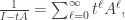
 is the
  denote the orthonormal matrix of normalized eigenvectors, so that
 ,
, 

 .
.![\frac{1}{I-tD_\Gamma}= P\cdot [\sum_{\ell=0}^\infty t^\ell A^\ell]\cdot P^{-1}.](https://s0.wp.com/latex.php?latex=%5Cfrac%7B1%7D%7BI-tD_%5CGamma%7D%3D+P%5Ccdot+%5B%5Csum_%7B%5Cell%3D0%7D%5E%5Cinfty+t%5E%5Cell+A%5E%5Cell%5D%5Ccdot+P%5E%7B-1%7D.&bg=ffffff&fg=323232&s=0&c=20201002)


 in
in  , we get,
![\sum_{j=0}^{n-1} \lambda_j^{-1}H(f)(\lambda_j^{-1}) = {\frac{1}{\pi}}\sum_{\ell=0}^\infty tr(A^\ell) [M(f)(\ell+1)+(-1)^\ell M(f^*)(\ell+1)],](https://s0.wp.com/latex.php?latex=%5Csum_%7Bj%3D0%7D%5E%7Bn-1%7D+%5Clambda_j%5E%7B-1%7DH%28f%29%28%5Clambda_j%5E%7B-1%7D%29+%3D+%7B%5Cfrac%7B1%7D%7B%5Cpi%7D%7D%5Csum_%7B%5Cell%3D0%7D%5E%5Cinfty+tr%28A%5E%5Cell%29+%5BM%28f%29%28%5Cell%2B1%29%2B%28-1%29%5E%5Cell+M%28f%5E%2A%29%28%5Cell%2B1%29%5D%2C&bg=ffffff&fg=323232&s=0&c=20201002)
 denotes the Hilbert transform
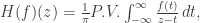 and
and  is the Mellin transform
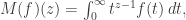
 denotes the negation,
  . Of course, if
  is even then
  , for all
  .
.  can be expressed in terms of the number of walks on the graph: If
  denotes the total number of walks of length
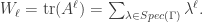
 , where
  is a quotient graph obtained from some subgroup
  . The examples are for graphs having a small number of vertices (no more than 12). For the most part, we also focused on regular graphs with small degree (no more than 5). They were all computed using
  .
.
 is a harmonic morphism. Let
  be adjacent vertices of
  and
and  “collapses” the edge (vertical)
  or (b)
  and the vertices
  and
and  are adjacent in
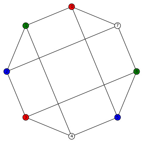
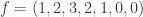
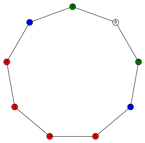
  the white vertex is not adjacent to the blue or red vertex, none of the harmonic colored graphs below can have a white vertex adjacent to a blue or red vertex.
 as the domain in this post. However, before we get to examples (obtained by using
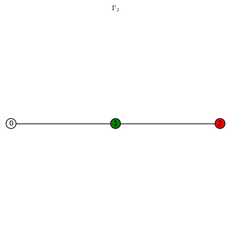
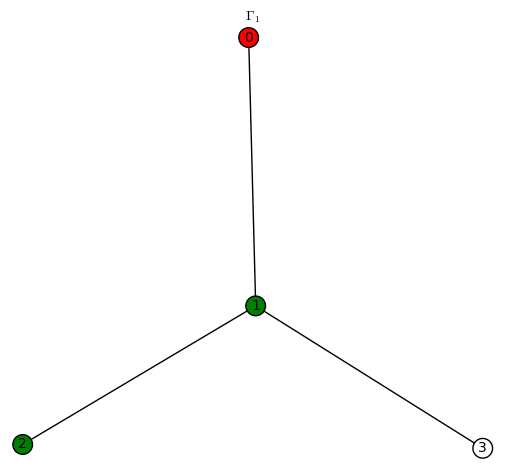
  be a harmonic morphism from a graph
  vertices to the path graph having
  vertices. Let
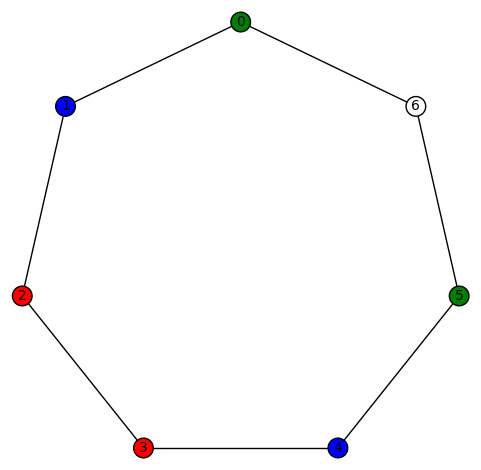
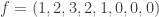
  be the coloring map (identified with an n-tuple whose coordinates are in
  ). Associated to f is a partition
 ![\Pi_f=[n_0,\dots,n_{k-1}]](https://s0.wp.com/latex.php?latex=%5CPi_f%3D%5Bn_0%2C%5Cdots%2Cn_%7Bk-1%7D%5D&bg=ffffff&fg=323232&s=0&c=20201002) of n (here
of n (here ![[...]](https://s0.wp.com/latex.php?latex=%5B...%5D&bg=ffffff&fg=323232&s=0&c=20201002) is a multi-set, so repetition is allowed but the ordering is unimportant):
is a multi-set, so repetition is allowed but the ordering is unimportant):  , where
  is the number of times j occurs in f. We call this the partition invariant of the harmonic morphism.
  ,
,  , with associated
 whose corresponding partitions agree,
  then we say
  and
and  examples!
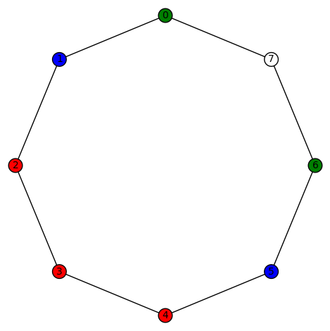
 , so we start with
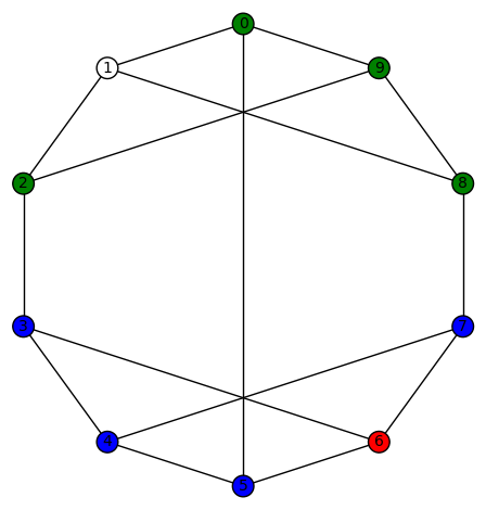
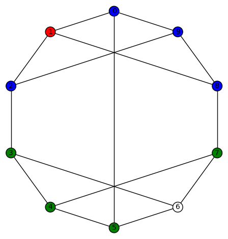
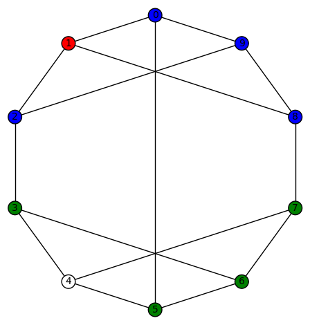
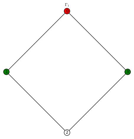
  . We indicate a harmonic morphism by a vertex coloring. An example of a harmonic morphism can be described in the plot below as follows:
  sends the red vertices in
  , plus that induced by
  and all of its cyclic permutations (4+6=10). This set of 6 permutations is closed under the automorphism of
 and all of its cyclic permutations (4+7=11). This set of 7 permutations is not closed under the automorphism of
  and all 7 of its cyclic permutations (total = 7+11 = 18).
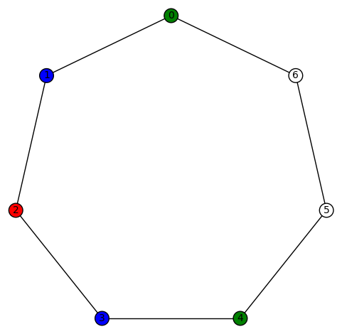
 and all of its cyclic permutations (4+8=12). This set of 8 permutations is not closed under the automorphism of
 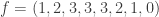 and all of its cyclic permutations (12+8=20). In addition, there is
  and all of its cyclic permutations (20+8 = 28). The latter set of 8 cyclic permutations of
  is closed under the transposition (0,3)(1,2) (total = 28).

 and all of its cyclic permutations (4+9=13). This set of 9 permutations is not closed under the automorphism of
  and all 9 of its cyclic permutations (9+13 = 22). This set of 9 permutations is not closed under the automorphism of
  and all 9 of its cyclic permutations (9+22 = 31). This set of 9 permutations is not closed under the automorphism of
  and all 9 of its cyclic permutations (total = 9+31 = 40).


 is the graph whose SageMath command is


 then, instead of showing a graph, I’ll list the edges (of course, the vertices are 0,1,…,11) and the SageMath command for it.
 , where
  .
. .
. .
. .
. .
. .
. .
. .
.
 and
and  are graphs then a map
  ) is a morphism provided
 and
and  then
then  is an edge in
  and
and  , where
  then
then  .
. is the dual map
  and
and  , then
  , an edge
  is called horizontal if
  and is called vertical if
  . We say that a graph morphism
  is a graph homomorphism if
  . Thus, a graph morphism is a homomorphism if it has no vertical edges.
 denote the star subgraph centered at the vertex v. A graph morphism
  is called harmonic if for all vertices
  , the quantity
 and mapping to the edge
  .
. sends the red vertices in
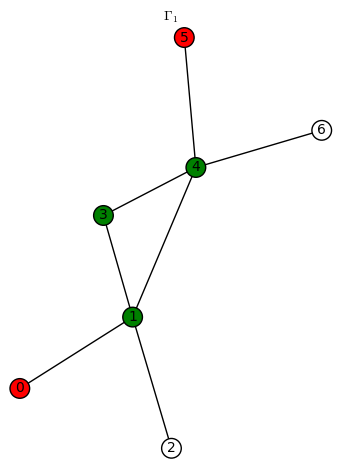

You must be logged in to post a comment.