Differential equations and SageMath

The files below were on my teaching page when I was a college teacher. Since I retired, they disappeared. Samuel Lelièvre found an archived copy on the web, so I’m posting them here.

The files are licensed under the Attribution-ShareAlike Creative Commons license.

  1. Partial fractions handout, pdf
  2. Introduction to matrix determinants handout, pdf
  3. Impulse-response handout, pdf
  4. Introduction to ODEs, pdf
  5. Initial value problems, pdf
  6. Existence and uniqueness, pdf
  7. Euler’s method for numerically approximating solutions to DEs, pdf.
    Includes both 1st order DE case (with Euler and improved Euler) and higher order DE and systems of DEs cases, without improved Euler.
  8. Direction fields and isoclines, pdf
  9. 1st order ODEs, separable and linear cases, pdf
  10. A falling body problem in Newtonian mechanics, pdf
  11. A mixing problem, pdf
  12. Linear ODEs, I, pdf
  13. Linear ODEs, II, pdf
  14. Undetermined coefficients for non-homogeneous 2nd order constant coefficient ODEs, pdf
  15. Variation of parameters for non-homogeneous 2nd order constant coefficient ODEs, pdf.
  16. Annihilator method for non-homogeneous 2nd order constant coefficient ODEs, pdf.
    I found students preferred (the more-or-less equivalent) undetermined coefficient method, so didn’t put much effort into these notes.
  17. Springs, I, pdf
  18. Springs, II, pdf
  19. Springs, III, pdf
  20. LRC circuits, pdf
  21. Power series methods, I, pdf
  22. Power series methods, II, pdf
  23. Introduction to Laplace transform methods, I, pdf
  24. Introduction to Laplace transform methods, II, pdf
  25. Lanchester’s equations modeling the battle between two armies, pdf
  26. Row reduction/Gauss elimination method for systems of linear equations, pdf.
  27. Eigenvalue method for homogeneous constant coefficient 2×2 systems of 1st order ODEs, pdf.
  28. Variation of parameters for first order non-homogeneous linear constant coefficient systems of ODEs, pdf.
  29. Electrical networks using Laplace transforms, pdf
  30. Separation of variables and the Transport PDE, pdf
  31. Fourier series, pdf.
  32. one-dimensional heat equation using Fourier series, pdf.
  33. one-dimensional wave equation using Fourier series, pdf.
  34. one-dimensional Schroedinger’s wave equation for a “free particle in a box” using Fourier series, pdf.
  35. All these lectures collected as one pdf (216 pages).
    While licensed Attribution-ShareAlike CC, in the US this book is in the public domain, as it was written while I was a US federal government employee as part of my official duties. A warning – it has lots of typos. The latest version, written with Marshall Hampton, is a JHUP book, much more polished, available on amazon and the JHUP website. Google “Introduction to Differential Equations Using Sage”.

Course review: pdf

Love, War, and Zombies, pdf
This set of slides is of a lecture I would give if there was enough time towards the end of the semester
Integral Calculus and SageMath

Long ago, using LaTeX I assembled a book on Calculus II (integral calculus), based on notes of mine, Dale Hoffman (which was written in word), and William Stein. I ran out of energy to finish it and the source files mostly disappeared from my HD. Recently, Samuel Lelièvre found a copy of the pdf of this book on the internet (you can download it here). It’s licensed under a Creative Commons Attribution 3.0 United States License. You are free to print, use, mix or modify these materials as long as you credit the original authors.

Table of Contents

0 Preface

1 The Integral
1.1 Area
1.2 Some applications of area
1.2.1 Total accumulation as “area”
1.2.2 Problems
1.3 Sigma notation and Riemann sums
1.3.1 Sums of areas of rectangles
1.3.2 Area under a curve: Riemann sums
1.3.3 Two special Riemann sums: lower and upper sums
1.3.4 Problems
1.3.5 The trapezoidal rule
1.3.6 Simpson’s rule and Sage
1.3.7 Trapezoidal vs. Simpson: Which Method Is Best?
1.4 The definite integral
1.4.1 The Fundamental Theorem of Calculus
1.4.2 Problems
1.4.3 Properties of the definite integral
1.4.4 Problems
1.5 Areas, integrals, and antiderivatives
1.5.1 Integrals, Antiderivatives, and Applications
1.5.2 Indefinite Integrals and net change
1.5.3 Physical Intuition
1.5.4 Problems
1.6 Substitution and Symmetry
1.6.1 The Substitution Rule
1.6.2 Substitution and definite integrals
1.6.3 Symmetry
1.6.4 Problems

2 Applications
2.1 Applications of the integral to area
2.1.1 Using integration to determine areas
2.2 Computing Volumes of Surfaces of Revolution
2.2.1 Disc method
2.2.2 Shell method
2.2.3 Problems
2.3 Average Values
2.3.1 Problems
2.4 Moments and centers of mass
2.4.1 Point Masses
2.4.2 Center of mass of a region in the plane
2.4.3 x-bar For A Region
2.4.4 y-bar For a Region
2.4.5 Theorems of Pappus
2.5 Arc lengths
2.5.1 2-D Arc length
2.5.2 3-D Arc length

3 Polar coordinates and trigonometric integrals
3.1 Polar Coordinates
3.2 Areas in Polar Coordinates
3.3 Complex Numbers
3.3.1 Polar Form
3.4 Complex Exponentials and Trigonometric Identities
3.4.1 Trigonometry and Complex Exponentials
3.5 Integrals of Trigonometric Functions
3.5.1 Some Remarks on Using Complex-Valued Functions

4 Integration techniques
4.1 Trigonometric Substitutions
4.2 Integration by Parts
4.2.1 More General Uses of Integration By Parts
4.3 Factoring Polynomials
4.4 Partial Fractions
4.5 Integration of Rational Functions Using Partial Fractions
4.6 Improper Integrals
4.6.1 Convergence, Divergence, and Comparison

5 Sequences and Series
5.1 Sequences
5.2 Series
5.3 The Integral and Comparison Tests
5.3.1 Estimating the Sum of a Series
5.4 Tests for Convergence
5.4.1 The Comparison Test
5.4.2 Absolute and Conditional Convergence
5.4.3 The Ratio Test
5.4.4 The Root Test
5.5 Power Series
5.5.1 Shift the Origin
5.5.2 Convergence of Power Series
5.6 Taylor Series
5.7 Applications of Taylor Series
5.7.1 Estimation of Taylor Series

6 Some Differential Equations
6.1 Separable Equations
6.2 Logistic Equation

7 Appendix: Integral tables

Gray codes

This is based on work done about 20 years ago with a former student Jim McShea.

Gray codes were introduced by Bell Labs physicist Frank Gray in the 1950s. As introduced, a Gray code is an ordering of the n-tuples in GF(2)^n = \{0,1\}^n such that two successive terms differ in only one position. A Gray code can be regarded as a Hamiltonian path in the cube graph. For example:

[[0, 0, 0], [1, 0, 0], [1, 1, 0], [0, 1, 0], [0, 1, 1], [1, 1, 1], [1, 0, 1], [0, 0, 1]]

These can be generalized to n-tuples of integers (mod m) in the obvious way.

Gray codes have several applications:

  • solving puzzles such as the Tower of Hanoi and the Brain [G],
  • analog-digital-converters (goniometers) [S],
  • Hamiltonian circuits in hypercubes [Gil] and Cayley graphs of Coxeter groups [CSW],
  • capanology (the study of bell-ringing) [W],
  • continuous space-filling curves [Gi],
  • classification of Venn diagrams [R],
  • design of communication codes,
  • and more (see Wikipedia).
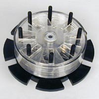
brain-puzzle

The Brain puzzle

Here's a SageMath/Python function for computing Gray codes.
def graycode(length,modulus):
    """
    Returns the n-tuple reverse Gray code mod m.


    EXAMPLES:
        sage: graycode(2,4)
        
        [[0, 0],
         [1, 0],
         [2, 0],
         [3, 0],
         [3, 1],
         [2, 1],
         [1, 1],
         [0, 1],
         [0, 2],
         [1, 2],
         [2, 2],
         [3, 2],
         [3, 3],
         [2, 3],
         [1, 3],
         [0, 3]]

    """
    n,m = length,modulus
    F = range(m)
    if n == 1:
        return [[i] for i in F]
    L = graycode(n-1, m)
    M = []
    for j in F:
        M = M+[ll+[j] for ll in L]
    k = len(M)
    Mr = [0]*m
    for i in range(m-1):
        i1 = i*int(k/m)
        i2 = (i+1)*int(k/m)
        Mr[i] = M[i1:i2]
    Mr[m-1] = M[(m-1)*int(k/m):]
    for i in range(m):
        if is_odd(i):
            Mr[i].reverse()
    M0 = []
    for i in range(m):
        M0 = M0+Mr[i]
    return M0


REFERENCES

[CSW] J. Conway, N. Sloane, and A. Wilks, “Gray codes and reflection groups”, Graphs and combinatorics 5(1989)315-325

[E] M. C. Er, “On generating the N-ary reflected Gray codes”, IEEE transactions on computers, 33(1984)739-741

[G] M. Gardner, “The binary Gray code”, in Knotted donuts and other mathematical entertainments, F. H. Freeman and Co., NY, 1986

[Gi] W. Gilbert, “A cube-filling Hilbert curve”, Math Intell 6 (1984)78

[Gil] E. Gilbert, “Gray codes and paths on the n-cube”, Bell System Technical Journal 37 (1958)815-826

[R] F. Ruskey, “A Survey of Venn Diagrams“, Elec. J. of Comb.(1997), and updated versions.

[S] Web page of T. Sillke

[W] A. White, “Ringing the cosets”, Amer. Math. Monthly 94(1987)721-746

How do I construct … in GAP?

This page is devoted to answering some basic questions along the line “How do I construct … in GAP?” You may view the html source code for the GAP commands without the output or GAP prompt.

Please send suggestions, additions, corrections to David Joyner.

This page itself is under construction…


Questions

How
do I construct a … group?

permutation
dihedral 
cyclicconjugacy classes of a
finitely presented

How
do I … a polynomial?
How do I find the … of a group
representation?
How do I compute an mod m, where A is …?
Given a group G, how do I compute … ?

Answers


    • permutation:
      To construct a permutation group, write down generators in disjoint cycle notation, put them in a list (i.e., surround them by square brackets), and the permutation group G generated by the cycles (1,2)(3,4) and (1,2,3):
gap> G:=Group((1,2)(3,4),(1,2,3));

Group([ (1,2)(3,4), (1,2,3) ])

This is of course a subgroup of the symmetric group S4 on 4 letters. Indeed, this G is in fact the alternating group on four letters, A4.

By virtue of the fact that the permutations generating G employ integers less than or equal to 4, this group G is a subgroup of the symmetric group S4 on 4 letters. Some permutation groups have special constructions:

gap> S4:=SymmetricGroup(4);
Sym( [ 1 .. 4 ] )
gap> A4:=AlternatingGroup(4);
Alt( [ 1 .. 4 ] )
gap> IsSubgroup(S4,G);
true
gap> IsSubgroup(A4,G);
true
gap> S3:=SymmetricGroup(3);
Sym( [ 1 .. 3 ] )
gap> IsSubgroup(S3,G);
false


    • dihedral
      To construct a dihedral group, use the special “DihedralGroup” command:
gap> G:=DihedralGroup(6);
gap> Size(G);
6
gap> f:=GeneratorsOfGroup( G );
[ f1, f2 ]
gap> f[1]^2; f[2]^3;
identity of ...
identity of ...
gap> f[1]^2= f[2]^3;
true


  • cyclic group
    To construct a cyclic group, you may construct integers mod n:

    gap> R:=ZmodnZ( 12);
    (Integers mod 12)
    gap> a:=Random(R);
    ZmodnZObj( 11, 12 )
    gap> 4*a;
    ZmodnZObj( 8, 12 )
    gap> b:=Random(R);
    ZmodnZObj( 9, 12 )
    gap> a+b;
    ZmodnZObj( 8, 12 )
    

    or use the special “CyclicGroup” command

    gap> G:=CyclicGroup(12);
    pc group of size 12 with 3 generators
    gap> a:=Random(G);
    f3^2
    gap> f:=GeneratorsOfGroup( G );
    [ f1, f2, f3 ]
    gap> f[1]^4;
    f3
    gap> f[1]^12;
    identity of ...


  • conjugacy:
    The conjugacy classes of a group G are computed using the “ConjugacyClasses” command. This is a list of classes {x^-1*g*x | x in G}.

    gap> G:=SL(2,7);
    SL(2,7)
    gap> CG:=ConjugacyClasses(G);
    [ [ [ Z(7)^0, 0*Z(7) ], [ 0*Z(7), Z(7)^0 ] ]^G,
      [ [ 0*Z(7), Z(7)^3 ], [ Z(7)^0, Z(7)^5 ] ]^G,
      [ [ 0*Z(7), Z(7)^4 ], [ Z(7)^5, Z(7)^5 ] ]^G,
      [ [ Z(7)^3, 0*Z(7) ], [ 0*Z(7), Z(7)^3 ] ]^G,
      [ [ 0*Z(7), Z(7)^3 ], [ Z(7)^0, Z(7)^2 ] ]^G,
      [ [ 0*Z(7), Z(7)^4 ], [ Z(7)^5, Z(7)^2 ] ]^G,
      [ [ 0*Z(7), Z(7)^3 ], [ Z(7)^0, 0*Z(7) ] ]^G,
      [ [ 0*Z(7), Z(7)^3 ], [ Z(7)^0, Z(7)^4 ] ]^G,
      [ [ 0*Z(7), Z(7)^3 ], [ Z(7)^0, Z(7) ] ]^G,
      [ [ Z(7)^4, 0*Z(7) ], [ 0*Z(7), Z(7)^2 ] ]^G,
      [ [ Z(7)^5, 0*Z(7) ], [ 0*Z(7), Z(7) ] ]^G ]
    gap> g:=Representative(CG[3]); Order(g);
    [ [ 0*Z(7), Z(7)^4 ], [ Z(7)^5, Z(7)^5 ] ]
    14
    gap> g:=Representative(CG[4]); Order(g);
    [ [ Z(7)^3, 0*Z(7) ], [ 0*Z(7), Z(7)^3 ] ]
    2
    gap> g:=Representative(CG[5]); Order(g);
    [ [ 0*Z(7), Z(7)^3 ], [ Z(7)^0, Z(7)^2 ] ]
    7
    gap> g:=Representative(CG[6]); Order(g);
    [ [ 0*Z(7), Z(7)^4 ], [ Z(7)^5, Z(7)^2 ] ]
    7
    gap>                            


  • presented
    To construct a finitely presented group in GAP, use the “FreeGroup” and “FpGroupPresentation” commands. Here is one example.

    gap> M12 := MathieuGroup( 12 );
    Group([ (1,2,3,4,5,6,7,8,9,10,11), (3,7,11,8)(4,10,5,6), (1,12)(2,11)(3,6)(4,8)(5,9)(7,10) ])
    gap> F := FreeGroup( "a", "b", "c" );
    free group on the generators [ a, b, c ]
    gap> words := [ F.1, F.2 ];
    [ a, b ]
    gap> P := PresentationViaCosetTable( M12, F, words );
    presentation with 3 gens and 10 rels of total length 97
    gap> TzPrintRelators( P );
    #I  1. c^2
    #I  2. b^4
    #I  3. a*c*a*c*a*c
    #I  4. a*b^2*a*b^-2*a*b^-2
    #I  5. a^11
    #I  6. a^2*b*a^-2*b^2*a*b^-1*a^2*b^-1
    #I  7. a*b*a^-1*b*a^-1*b^-1*a*b*a^-1*b*a^-1*b^-1
    #I  8. a^2*b*a^2*b^2*a^-1*b*a^-1*b^-1*a^-1*b^-1
    #I  9. a*b*a*b*a^2*b^-1*a^-1*b^-1*a*c*b*c
    #I  10. a^4*b*a^2*b*a^-2*c*a*b*a^-1*c
    gap> G := FpGroupPresentation( P );
    fp group on the generators [ a, b, c ]
    gap> RelatorsOfFpGroup( G );  
    [ c^2, b^4, a*c*a*c*a*c, a*b^-2*a*b^-2*a*b^-2, a^11, a^2*b*a^-2*b^-2*a*b^-1*a^2*b^-1, a*b*a^-1*b*a^-1*b^-1*a*b*a^-1*b*a^-1*b^-1,
      a^2*b*a^2*b^-2*a^-1*b*a^-1*b^-1*a^-1*b^-1, a*b*a*b*a^2*b^-1*a^-1*b^-1*a*c*b*c, a^4*b*a^2*b*a^-2*c*a*b*a^-1*c ]
    gap> Size(M12);
    95040
    gap> Size(G);
    95040
    gap> IsomorphismGroups(G,M12); 
    ????????
    

    The last command is computationally intensive and requires more than the default memory allocation of 256M of RAM.

    Here is another example.

    gap> F := FreeGroup( "a", "b");
    free group on the generators [ a, b ]
    gap> G:=F/[F.1^2,F.2^3,F.1*F.2*F.1^(-1)*F.2^(-1)];
    fp group on the generators [ a, b ]
    gap> Size(G);
    6


  • rref
    The key command for row reduction is “TriangulizeMat”. The following example illustrates the syntax.

    gap> M:=[[1,2,3,4,5],[1,2,1,2,1],[1,1,0,0,0]];
    [ [ 1, 2, 3, 4, 5 ], [ 1, 2, 1, 2, 1 ], [ 1, 1, 0, 0, 0 ] ]
    gap> TriangulizeMat(M);
    gap> M;
    [ [ 1, 0, 0, -1, 1 ], [ 0, 1, 0, 1, -1 ], [ 0, 0, 1, 1, 2 ] ]
    gap> Display(M);
    [ [   1,   0,   0,  -1,   1 ],
      [   0,   1,   0,   1,  -1 ],
      [   0,   0,   1,   1,   2 ] ]
    gap> M:=Z(3)^0*[[1,2,3,4,5],[1,2,1,2,1],[1,1,0,0,0]];
    [ [ Z(3)^0, Z(3), 0*Z(3), Z(3)^0, Z(3) ],
      [ Z(3)^0, Z(3), Z(3)^0, Z(3), Z(3)^0 ],
      [ Z(3)^0, Z(3)^0, 0*Z(3), 0*Z(3), 0*Z(3) ] ]
    gap> TriangulizeMat(M);
    gap> Display(M);
     1 . . 2 1
     . 1 . 1 2
     . . 1 1 2
    gap>


  • kernel:
    There are different methods for matrices over the integers and matrices over a field. For integer entries, related commands include “NullspaceIntMat” and “SolutionNullspaceIntMat” in section 25.1 “Linear equations over the integers and Integral Matrices” of the reference manual.

    gap> M:=[[1,2,3],[4,5,6],[7,8,9]];
    [ [ 1, 2, 3 ], [ 4, 5, 6 ], [ 7, 8, 9 ] ]
    gap> NullspaceIntMat(M);
    [ [ 1, -2, 1 ] ]
    gap> SolutionNullspaceIntMat(M,[0,0,1]);
    [ fail, [ [ 1, -2, 1 ] ] ]
    gap> SolutionNullspaceIntMat(M,[0,0,0]);
    [ [ 0, 0, 0 ], [ [ 1, -2, 1 ] ] ]
    gap> SolutionNullspaceIntMat(M,[1,2,3]);
    [ [ 1, 0, 0 ], [ [ 1, -2, 1 ] ] ]


    Here (0,0,1) is not in the image of M
    (under v-> v*M) but (0,0,0) and (1,2,3) are.

    For field entries, related commands include “NullspaceMat” and “TriangulizedNullspaceMat” in section 24.6 “Matrices Representing Linear Equations and the Gaussian Algorithm”
    of the reference manual.

    gap> M:=[[1,2,3],[4,5,6],[7,8,9]];
    [ [ 1, 2, 3 ], [ 4, 5, 6 ], [ 7, 8, 9 ] ]
    gap> NullspaceMat(M);
    [ [ 1, -2, 1 ] ]
    gap> TriangulizedNullspaceMat(M);
    [ [ 1, -2, 1 ] ]
    gap> M:=[[1,2,3,1,1],[4,5,6,1,1],[7,8,9,1,1],[1,2,3,1,1]];
    [ [ 1, 2, 3, 1, 1 ], [ 4, 5, 6, 1, 1 ], [ 7, 8, 9, 1, 1 ], 
      [ 1, 2, 3, 1, 1 ] ]
    gap> NullspaceMat(M);
    [ [ 1, -2, 1, 0 ], [ -1, 0, 0, 1 ] ]
    gap> TriangulizedNullspaceMat(M);
    [ [ 1, 0, 0, -1 ], [ 0, 1, -1/2, -1/2 ] ]


  • characteristic polynomial:
    Please see section 24.12.1 of the GAP reference manual for examples of characteristic polynomial of a square matrix (“CharacteristicPolynomial”) and section 56.3 for examples of the “characteristic polynomial” (called a “TracePolynomial”) of an element of a field extension.


  • character:
    GAP contains very extensive character theoretic functions and data libraries (including an interface the character table in the Atlas). Here is just one simple example.

    gap> G:=Group((1,2)(3,4),(1,2,3));
    Group([ (1,2)(3,4), (1,2,3) ])
    gap> T:=CharacterTable(G);
    CharacterTable( Alt( [ 1 .. 4 ] ) )
    gap> Display(T);
    CT1
    
         2  2  2  .  .
         3  1  .  1  1
    
           1a 2a 3a 3b
        2P 1a 1a 3b 3a
        3P 1a 2a 1a 1a
    
    X.1     1  1  1  1
    X.2     1  1  A /A
    X.3     1  1 /A  A
    X.4     3 -1  .  .
    
    A = E(3)^2
      = (-1-ER(-3))/2 = -1-b3
    gap> irr:=Irr(G);
    [ Character( CharacterTable( Alt( [ 1 .. 4 ] ) ), [ 1, 1, 1, 1 ] ),
      Character( CharacterTable( Alt( [ 1 .. 4 ] ) ), [ 1, 1, E(3)^2, E(3) ] ),
      Character( CharacterTable( Alt( [ 1 .. 4 ] ) ), [ 1, 1, E(3), E(3)^2 ] ),
      Character( CharacterTable( Alt( [ 1 .. 4 ] ) ), [ 3, -1, 0, 0 ] ) ]
    gap> Display(irr);
    [ [       1,       1,       1,       1 ],
      [       1,       1,  E(3)^2,    E(3) ],
      [       1,       1,    E(3),  E(3)^2 ],
      [       3,      -1,       0,       0 ] ]
    gap> chi:=irr[2]; gamma:=CG[3]; g:=Representative(gamma); g^chi;
    Character( CharacterTable( Alt( [ 1 .. 4 ] ) ), [ 1, 1, E(3)^2, E(3) ] )
    (1,2,3)^G
    (1,2,3)
    E(3)^2


    For further details and examples, see chapters 6972 of the GAP reference manual.

  • brauer:
    Just a simple example of what GAP can do here. To construct a Brauer character table:

    gap> G:=Group((1,2)(3,4),(1,2,3));
    Group([ (1,2)(3,4), (1,2,3) ])
    gap> irr:=IrreducibleRepresentations(G,GF(7));
    [ [ (1,2)(3,4), (1,2,3) ] -> [ [ [ Z(7)^0 ] ], [ [ Z(7)^0 ] ] ],
      
    [ (1,2)(3,4), (1,2,3) ] -> [ [ [ Z(7)^0 ] ], [ [ Z(7)^4 ] ] ],
      
    [ (1,2)(3,4), (1,2,3) ] -> [ [ [ Z(7)^0 ] ], [ [ Z(7)^2 ] ] ],
      
    [ (1,2)(3,4), (1,2,3) ] -> [
          
    [ [ 0*Z(7), Z(7)^3, Z(7)^0 ], [ 0*Z(7), Z(7)^3, 0*Z(7) ], 
    [ Z(7)^0, Z(7)^3, 0*Z(7) ] ],
          [ [ 0*Z(7), Z(7)^0, 0*Z(7) ], 
    [ 0*Z(7), 0*Z(7), Z(7)^0 ], [ Z(7)^0, 0*Z(7), 0*Z(7) ] ]
         
    ] ]
    gap> brvals := List(irr,chi-> List(ConjugacyClasses(G),c->
    BrauerCharacterValue(Image(chi, Representative(c)))));
    [ [ 1, 1, 1, 1 ], [ 1, 1, E(3)^2, E(3) ], [ 1, 1, E(3), E(3)^2 ], 
    [ 3, -1, 0, 0 ] ]
    gap> Display(brvals);
    [ [       1,       1,       1,       1 ],
      
    [       1,       1,  E(3)^2,    E(3) ],
      
    [       1,       1,    E(3),  E(3)^2 ],
      
    [       3,      -1,       0,       0 ] ]
    gap>                                               
    

    List(ConjugacyClasses(G),c->BrauerCharacterValue(Image(chi, Representative(c)))));
    #Display(brvals);
    T:=CharacterTable(G);
    Display(T);
    –>


  • polynomial
    There are various ways to construct a polynomial in GAP.

    gap> Pts:=Z(7)^0*[1,2,3];
    [ Z(7)^0, Z(7)^2, Z(7) ]
    gap> Vals:=Z(7)^0*[1,2,6];
    [ Z(7)^0, Z(7)^2, Z(7)^3 ]
    gap> g:=InterpolatedPolynomial(GF(7),Pts,Vals);
    Z(7)^5*x_1^2+Z(7)
    

    Or:

    gap> p:=3;; F:=GF(p);;
    gap> R:=PolynomialRing(F,["x1","x2"]);
    PolynomialRing(..., [ x1, x2 ])
    gap> vars:=IndeterminatesOfPolynomialRing(R);;
    gap> x1:=vars[1]; x2:=vars[2];
    x1
    x2
    gap> p:=x1^5-x2^5;
    x1^5-x2^5
    gap> DivisorsMultivariatePolynomial(p,R);
    [ x1^4+x1^3*x2+x1^2*x2^2+x1*x2^3+x2^4, x1-x2 ]
    

    Or:

    gap> x:=X(Rationals);
    x_1
    gap> f:=x+x^2+1;
    x_1^2+x_1+1
    gap> Value(f,[x],[1]);
    3


  • factor
    To factor a polynomial in GAP, there is one command for univariate polynomials (“Factors”) and another command for multivariate polynomials (“DivisorsMultivariatePolynomial”). For a factoring a univariate polynomial, GAP provides only methods over finite fields and over subfields of cyclotomic fields. Please see the examples given in section 64.10 “Polynomial Factorization” for more details. For multivariate polynomials, a very slow algorithm has been implemented in GAP and an interface to a very fast algorithm in Singular has been implemented for those who have both Singular and the GAP Singular package installed. The former of these was illustrated above in “polynomial” above. (Again, the ground field must be a finite field or a subfields of cyclotomic fields.) For the latter, please see the example in the (GAP-)Singular manual FactorsUsingSingularNC.


  • roots
    There are some situations where GAP can find the roots of a polynomial but GAP does not do this generally. (The roots must generate either a finite field or a subfield of a cyclotomic field.) However, there is a package called RadiRoot which must be installed which does help to do this for polynomials with rational coefficients (radiroot itself requires other packages to be installed; please see the webpage for more details). The “Factors” command actually has an option which allows you to increase the groundfield so that a factorization actually returns the roots. Please see the examples given in section 64.10 “Polynomial Factorization” for more details. Here is a second approach.

    gap> p:=3; n:=4; F:=GF(p^n); c:=Random(F); r:=2;
    3
    4
    GF(3^4)
    Z(3^4)^79
    2
    gap>  x:=X(F,1); f:=x^r-c*x+c-1;
    x_1
    x_1^2+Z(3^4)^39*x_1+Z(3^4)^36
    gap>  F_f:=FieldExtension( F, f );
    AsField( GF(3^4), GF(3^8) )
    gap>  alpha:=RootOfDefiningPolynomial(F_f);
    Z(3^4)^36
    gap> Value(f,[x],[alpha]);
    0*Z(3)


    Here is a third. First, enter the following program

    RootOfPolynomial:=function(f,R)
     local F0,Ff,a;
     F0:=CoefficientsRing(R);
     Ff:=FieldExtension(F0,f);
     a:=RootOfDefiningPolynomial(Ff);
     return a;
    end;
    

    Here’s how this can be used to find a root:

    gap> F:=Rationals;
    Rationals
    gap> x:=X(F,1); f:=x^2+x+1;
    x_1
    x_1^2+x_1+1
    gap> R:=PolynomialRing( F, [ x ]);
    PolynomialRing(..., [ x_1 ])
    gap> a:=RootOfPolynomial(f,R);
    E(3)
    gap> # check:
    gap> Value(f,[x],[a]);
    0
    

    Related links:

    1. In the GAP Forum: Hensel lifting discussion.
    2. In the manual, Galois groups.

  • evaluate:
    The relevant command is “Value”. There are several examples already on this page. For others, please see the examples given in section 64.7 Multivariate polynomials of the manual. For sparse uivariate polynomials, there is also the command “ValuePol” in section 23.6 of the manual.


  • integer power
    This is easy and intuitive:

    gap> a:=1000; n:=100000; m:=123;
    1000
    100000
    123
    gap> a^n mod m;
    1


  • matrix power:
    This too is easy and intuitive:

    gap> A:=[[1,2],[3,4]]; n:=100000; m:=123;
    [ [ 1, 2 ], [ 3, 4 ] ]
    100000
    123
    gap> A^n mod m;
    [ [ 1, 41 ], [ 0, 1 ] ]
    

  • polynomial power
    GAP allows you to do arithmetic over the polynomial ring R[x], where R = Z/nZ (where n is a positive integer). Here’s an example.

    gap> Z4:=ZmodnZ(4);
    (Integers mod 4)
    gap> R:=UnivariatePolynomialRing(Z4,1);
    PolynomialRing(..., [ x ])
    gap> x:=IndeterminatesOfPolynomialRing(R)[1];
    x
    gap> I:=TwoSidedIdealByGenerators( R,[x^8-x^0]);
    two-sided ideal in PolynomialRing(..., [ x ]), (1 generators)
    gap> gen:=x^8-x^0;
    x8-ZmodnZObj(1,4)
    gap> QuotientRemainder(R,x^8,gen);
    [ ZmodnZObj(1,4), ZmodnZObj(1,4) ]
    gap> QuotientRemainder(R,x^15,gen);
    [ x^7, x^7 ]
    gap> QuotientRemainder(R,x^15+x^8,gen);
    [ x^7+ZmodnZObj(1,4), x^7+ZmodnZObj(1,4) ]
    gap> PowerMod( R, x+x^0, 15, gen );
    ZmodnZObj(0,4)
    gap> PowerMod( R, x, 15, gen );
    x^7


  • Groebner basis
    GAP’s Groebner bases algorithms are relatively slow and are included mostly for simple examples and for teaching purposes. However, a GAP interface to a very fast algorithm in Singular has been implemented for those who have both Singular and the GAP Singular package installed. The former of these is illustrated in section 64.17 Groebner bases of the GAP manual. For the latter, please see the example in the (GAP-)Singular manual GroebnerBasis.


  • normal subgroup:
    Here is an example:

    gap> G := AlternatingGroup( 5 );
    Group( (1,2,5), (2,3,5), (3,4,5) )
    gap> normal := NormalSubgroups( G );
    [ Subgroup( Group( (1,2,5), (2,3,5), (3,4,5) ), [  ] ), 
      Subgroup( Group( (1,2,5), (2,3,5), (3,4,5) ), 
        [ (1,2)(3,4), (1,3)(4,5), (1,4)(2,3) ] ) ]
    

    Related links:

    1. Please see Volkmar Felsch’s GAP Forum response to a related question.
    2. The xgap package (or, on a mac, Gap.app) displays subgroup lattices graphically.

  • abelian subgroup
    One idea to compute all the abelian subgroups is to compute all the subgroups then “filter” out the abelian ones. Here is an illustration, taked from a GAP Forum response Volkmar Felsch.

    gap> G := AlternatingGroup( 5 );
    Group( (1,2,5), (2,3,5), (3,4,5) )
    gap> classes := ConjugacyClassesSubgroups( G );
    [ ConjugacyClassSubgroups( Group( (1,2,5), (2,3,5), 
        (3,4,5) ), Subgroup( Group( (1,2,5), (2,3,5), (3,4,5) ), [  ] ) ),
      ConjugacyClassSubgroups( Group( (1,2,5), (2,3,5), 
        (3,4,5) ), Subgroup( Group( (1,2,5), (2,3,5), (3,4,5) ), 
        [ (2,3)(4,5) ] ) ), ConjugacyClassSubgroups( Group( (1,2,5), 
        (2,3,5), (3,4,5) ), Subgroup( Group( (1,2,5), (2,3,5), (3,4,5) ), 
        [ (3,4,5) ] ) ), ConjugacyClassSubgroups( Group( (1,2,5), 
        (2,3,5), (3,4,5) ), Subgroup( Group( (1,2,5), (2,3,5), (3,4,5) ), 
        [ (2,3)(4,5), (2,4)(3,5) ] ) ), ConjugacyClassSubgroups( Group( 
        (1,2,5), (2,3,5), (3,4,5) ), Subgroup( Group( (1,2,5), (2,3,5), 
        (3,4,5) ), [ (1,2,3,4,5) ] ) ), ConjugacyClassSubgroups( Group( 
        (1,2,5), (2,3,5), (3,4,5) ), Subgroup( Group( (1,2,5), (2,3,5), 
        (3,4,5) ), [ (3,4,5), (1,2)(4,5) ] ) ), 
      ConjugacyClassSubgroups( Group( (1,2,5), (2,3,5), 
        (3,4,5) ), Subgroup( Group( (1,2,5), (2,3,5), (3,4,5) ), 
        [ (1,2,3,4,5), (2,5)(3,4) ] ) ), ConjugacyClassSubgroups( Group( 
        (1,2,5), (2,3,5), (3,4,5) ), Subgroup( Group( (1,2,5), (2,3,5), 
        (3,4,5) ), [ (2,3)(4,5), (2,4)(3,5), (3,4,5) ] ) ), 
      ConjugacyClassSubgroups( Group( (1,2,5), (2,3,5), (3,4,5) ), Group( 
        (1,2,5), (2,3,5), (3,4,5) ) ) ]
    gap> cl := classes[4];
    ConjugacyClassSubgroups( Group( (1,2,5), (2,3,5), 
    (3,4,5) ), Subgroup( Group( (1,2,5), (2,3,5), (3,4,5) ), 
    [ (2,3)(4,5), (2,4)(3,5) ] ) )
    gap> length := Size( cl );
    5
    gap> rep := Representative( cl );
    Subgroup( Group( (1,2,5), (2,3,5), (3,4,5) ), 
    [ (2,3)(4,5), (2,4)(3,5) ] )
    gap> order := Size( rep );
    4
    gap> IsAbelian( rep );
    true
    gap> abel := Filtered( classes, cl -> IsAbelian( Representative( cl ) ) );
    [ ConjugacyClassSubgroups( Group( (1,2,5), (2,3,5), 
        (3,4,5) ), Subgroup( Group( (1,2,5), (2,3,5), (3,4,5) ), [  ] ) ),
      ConjugacyClassSubgroups( Group( (1,2,5), (2,3,5), 
        (3,4,5) ), Subgroup( Group( (1,2,5), (2,3,5), (3,4,5) ), 
        [ (2,3)(4,5) ] ) ), ConjugacyClassSubgroups( Group( (1,2,5), 
        (2,3,5), (3,4,5) ), Subgroup( Group( (1,2,5), (2,3,5), (3,4,5) ), 
        [ (3,4,5) ] ) ), ConjugacyClassSubgroups( Group( (1,2,5), 
        (2,3,5), (3,4,5) ), Subgroup( Group( (1,2,5), (2,3,5), (3,4,5) ), 
        [ (2,3)(4,5), (2,4)(3,5) ] ) ), ConjugacyClassSubgroups( Group( 
        (1,2,5), (2,3,5), (3,4,5) ), Subgroup( Group( (1,2,5), (2,3,5), 
        (3,4,5) ), [ (1,2,3,4,5) ] ) ) ]
    

  • homology
    This depends on how the group is given. For example, suppose that G is a permutation group with generators genG and H is a permutation group with generators genH. To find a homomorphism from G to H, one may use the “GroupHomomorphismByImages” or “GroupHomomorphismByImagesNC” commands. For examples of the syntax, please see section 38.1 Creating Group Homomorphisms. Here’s an illustration of how to convert a finitely presented group into a permutation group.

    gap> p:=7;
    7
    gap> G:=PSL(2,p);
    Group([ (3,7,5)(4,8,6), (1,2,6)(3,4,8) ])
    gap> H:=SchurCover(G);
    fp group of size 336 on the generators [ f1, f2, f3 ]
    gap> iso:=IsomorphismPermGroup(H);
    [ f1, f2, f3 ] -> [ (1,2,4,3)(5,9,7,10)(6,11,8,12)(13,14,15,16),
      (2,5,6)(3,7,8)(11,13,14)(12,15,16), (1,4)(2,3)(5,7)(6,8)(9,10)(11,12)(13,
        15)(14,16) ]
    gap> H0:=Image(iso);                       # 2-cover of PSL2
    Group([ (1,2,4,3)(5,9,7,10)(6,11,8,12)(13,14,15,16),
      (2,5,6)(3,7,8)(11,13,14)(12,15,16), (1,4)(2,3)(5,7)(6,8)(9,10)(11,12)(13,
        15)(14,16) ])
    gap> IdGroup(H0);
    [ 336, 114 ]
    gap> IdGroup(SL(2,7));
    [ 336, 114 ]
    gap>                
    

  • semi-direct product(Contributed by Nilo de Roock):
    As you can easily verify, D8 is isomorphic to C2:C4. Or in GAP…

    N:=CyclicGroup(IsPermGroup,4);
    G:=CyclicGroup(IsPermGroup,2);
    AutN:=AutomorphismGroup(N);
    f:=GroupHomomorphismByImages(G,AutN,GeneratorsOfGroup(G),[Elements(AutN)[2]]);
    NG:=SemidirectProduct(G,f,N);
    

    Verify with

    StructureDescription(NG);
    

  • semi-direct products(Contributed by Nilo de Roock):
    The following shows how to construct all non-abelian groups of order 12 as semi-direct products. These products are not trivial yet small enough to verify by hand.

    #D12 = (C2 x C2) : C3
    G1:=CyclicGroup(IsPermGroup,2);
    G2:=CyclicGroup(IsPermGroup,2);
    G:=DirectProduct(G1,G2);
    N:=CyclicGroup(IsPermGroup,3);
    AutN:=AutomorphismGroup(N);
    f:=GroupHomomorphismByImages(G,AutN,[Elements(G)[1],Elements(G)[2],Elements(G)[3],Elements(G)[4]],[Elements(AutN)[1],Elements(AutN)[2],Elements(AutN)[1],Elements(AutN)[2]]);
    NG:=SemidirectProduct(G,f,N);
    Print(str(NG));
    Print("\n");
    
    #T = C4 : C3
    G:=CyclicGroup(IsPermGroup,4);
    N:=CyclicGroup(IsPermGroup,3);
    AutN:=AutomorphismGroup(N);
    f:=GroupHomomorphismByImages(G,AutN,[Elements(G)[1],Elements(G)[2],Elements(G)[3],Elements(G)[4]],[Elements(AutN)[1],Elements(AutN)[2],Elements(AutN)[1],Elements(AutN)[2]]);
    NG:=SemidirectProduct(G,f,N);
    Print(str(NG));
    Print("\n");
    
    #A4 = C3 : (C2 x C2)
    G:=CyclicGroup(IsPermGroup,3);
    N1:=CyclicGroup(IsPermGroup,2);
    N2:=CyclicGroup(IsPermGroup,2);
    N:=DirectProduct(G1,G2);
    AutN:=AutomorphismGroup(N);
    f:=GroupHomomorphismByImages(G,AutN,[Elements(G)[1],Elements(G)[2],Elements(G)[3]],[Elements(AutN)[1],Elements(AutN)[4],Elements(AutN)[5]]);
    NG:=SemidirectProduct(G,f,N);
    Print(str(NG));
    Print("\n");
    

  • cohomology
    GAP will compute the Schur multiplier H2(G,C) using the
    “AbelianInvariantsMultiplier” command. Here is an example showing how to find H2(A5,C), where A5 is the alternating group on 5 letters.

    gap> A5:=AlternatingGroup(5);
    Alt( [ 1 .. 5 ] )
    gap> AbelianInvariantsMultiplier(A5);
    [ 2 ]
    

    So, H2(A5,C) is Z/2Z.

    Related links:

    1. See section 37.23 and section 37.24 of the GAP manual.
    2. See D. Holt’s GAP package cohomolo.

Mathematics of zombies

What do you do if there is a Zombie attack? Can mathematics help? This page is (humorously) dedicated to collecting links to papers or blog posted related to the mathematical models of Zombies.


George Romero’s 1968 Night of the Living Dead, now in the public domain, introduced reanimated ghouls, otherwise known as zombies, which craved live human flesh. Romero’s script was insired on Richard Matheson’s I Am Legend. In Romero’s version, the zombies could be killed by destroying the zombie’s brain. A dead human could, in some cases be “reanimated,” turning into a zombie. These conditions are modeled mathematically in several papers, given below.

  1. When Zombies Attack! Mathematical Modelling of a Zombie Outbreak!, paper by Mathematicians at the University of Ottawa, Philip Munz, Ioan Hudea, Joe Imad and Robert J. Smith? (yes, his last name is spelled “Smith?”).
  2. youtube video 28 Minutes Later – The Maths of Zombies , made by Dr James Grime (aka, “siningbanana”), which references the above paper.
  3. Epidemics in the presence of social attraction and repulsion, Oct 2010 Zombie paper by Evelyn Sander and Chad M. Topaz.
  4. Statistical Inference in a Zombie Outbreak Model, slides for a talk given by Des Higman, May 2010.
  5. Mathematics kills zombies dead!, 08/17/2009 blog post by “Zombie Research Society Staff”.
  6. The Mathematics of Zombies, August 18, 2009 blog post by Mike Elliot.
  7. Love, War and Zombies – Systems of Differential Equations using Sage, April 2011 slides by David Joyner. Sage commands for Love, War and Zombies talk. This was given as a Project Mosaic/M-cast broadcast.
  8. Public domain 1968 film Night of the Living Dead by George Romero.

Zombies and Mathematics

What do you do if there is a Zombie attack? Can mathematics help? This post is (humorously) dedicated to collecting links to papers or blog posted related to the mathematical models of Zombies.

George Romero‘s 1968 Night of the Living Dead, now in the public domain, introduced reanimated ghouls, otherwise known as zombies, which craved live human flesh. Romero’s script was insired on Richard Matheson’s I Am Legend. In Romero’s version, the zombies could be killed by destroying the zombie’s brain. A dead human could, in some cases be “reanimated,” turning into a zombie. These conditions are modeled mathematically in several papers, given below.

Public domain 1968 film Night of the Living Dead by George Romero.

Sage and the future of mathematics

I am not a biologist nor a chemist, and maybe neither are you, but suppose we were. Now, if I described a procedure, in “standard” detail, to produce a result XYZ, you would (based on your reasonably expected expertise in the field), follow the steps you believe were described and either reproduce XYZ or, if I was mistaken, not be able to reproduce XYZ. This is called scientific reproducibility. It is cructial to what I believe is one of the fundamental principles of science, namely Popper’s Falsifiability Criterion.

More and more people are arguing, correctly in my opinion, that in the computational realm, in particular in mathematical research which uses computational experiments, that much higher standards are needed. The Ars Technica article linked above suggests that “it’s time for a major revision of the scientific method.” Also, Victoria Stodden argues one must “facilitate reproducibility. Without this data may be open, but will remain de facto in the ivory tower.” The argument basically is that to reproduce computational mathematical experiments is unreasonably difficult, requiring more that a reasonable expertise. These days, it may in fact (unfortunately) require purchasing very expensive software, or possessing of very sophisticated programming skills, accessibility to special hardware, or (worse) guessing parameters and programming procedures only hinted at by the researcher.

Hopefully, Sage can play the role of a standard bearer for such computational reproducibility. Sage is free, open source and there is a publically available server it runs on (sagenb.org).

What government agencies should require such reproducibility? In my opinion, all scientific funding agencies (NSF, etc) should follow these higher standards of computational accountability.

Copyright law as it pertains to mathematics and mathematical software

Disclaimer: I am not a lawyer and this is not to be construed as legal advice. However, I find copyright law very interesting but complicated and wrote this only to try to explain some of the simpler aspects of copyright law which pertain to mathematical scholars.

This is a brief survey on some aspects of federal copyright law, as it pertains to mathematicians. (By mathematician, which we mean teachers or scholarly researchers at a non-profit educational institute; generally, the more commercial the enterprise, the more complicated the law is governing it. This small survey only discusses the simplest aspects.) It does not cover other aspects of intellectual property law, such as laws governing patents, trade secrets, and so on (see for example, [K]). We have used the excellent book [L] by Leaffer as a basis for this survey. Copyright law is very complex [US] but, I hope, this post shows that many parts of copyright law which pertain to mathematicians, is relatively uncomplicated.

U.S. copyright law applies to writings, or works ‘fixed in a tangible medium of expression’, produced by an author. For this article, we assume the author is a U. S. citizen and the work was produced on U. S. soil. However, a ‘writing’ is not assumed to be human-readable, so, for example, a software program in executable binary form, or ‘object code’, is included [L], section 3.06. The owner of the copyright of a work has the exclusive right for

  • reproduce or copy the work,
  • prepare derivative works,
  • distribute the work,
  • perform the work publicly,
  • display the work publicly.

Before explaining these terms, exceptions to these rights, and how these rights relate especially to mathematical works, we discuss works for which copyright law cannot be applied. The law is designed to protect creative written works.

  • Ideas are generally not subject to copyright. From section 102 of [US]:In no case does copyright protection for an original work of authorship extend to any idea, procedure, process, system, method of operation, concept, principle, or discovery, regardless of the form in which it is described, explained, illustrated, or embodied in such work.
  • An unoriginal work, or a work ‘mechanically produced’, say by a computer program whose use requires no originality, are not copyrightable (more precisely, are not subject to a separate copyright – the program could, for example, output copyrighted elements). For example, the output of an automatic theorem proving program is not copyrightable. On the other hand, the output of an image processing program which takes an image and applies a de-noising algorithm is a “mechanical” derivation of the original image, so the copyright is the same as that of the original.
  • Facts are is not copyrightable. It doesn’t matter how much money or man power it took to discover, collect, or obtain it. (However, there are various laws which can be used to protect such intellectual property, such as trade secret laws.) For example, you cannot copyright a theorem, such Fermat’s Last Theorem, as it is a fact.
    Indeed, section 102(b) of the copyright law (chapter 1, section 102 in [US]) says:

    In no case does copyright protection for an original work of authorship extend to any idea, procedure, process, system, method of operation, concept, principle, or discovery, regardless of the form in which it is described, explained, illustrated, or embodied in such work.

    I have put `discovery’ in bold for emphasis.

    In some cases, a creative arrangement of data is copyrightable, for example, statistical data displayed in an unusual way, even if the data itself is not.

  • Works in the public domain (in particular most ‘official’ works by the U. S. government), are not copyrightable. All written works eventually pass into the public domain. Due to the variety of copyright laws which have been passed in the United States over the years, the duration of copyright depends on when the work was written, if it is a joint work (or a ‘work for hire’) or not, and various other factors. In fact, all of chapter 3 or the copyright code [US] is devoted to to duration, so it is complicated. However, life plus 70 years should apply in most cases.
    From section 302(a) of [US]:
  • In General. — Copyright in a work created on or after January 1, 1978, subsists from its creation and, except as provided by the following subsections, endures for a term consisting of the life of the author and 70 years after the author’s death.

For the owner of a creative mathematical work, whether it is an article or a piece of software, we explain next what these rights mean.

  • Reproduction: A reproduction is to fix a copy in a tangible and relatively permanent form, such as a xerox copy or a file on a computer (though a copy stored in your cache is exempted). Aside from non-profit, educational, government, or ‘fair use’, the copyright holder has the sole right to make unlimited copies of the work. For example, if you publish a paper or book, you often sign over your copyright to a publisher. If anyone could make a copy of your article freely, the commercial interest of the publisher would disappear. Similarly, if you wrote a mathematical software program which you wanted to market, you would want to restrict the copies of the program to those who paid for it. A research paper downloaded from the internet and then emailed to a colleague is an example of a reproduction.However, there is a ‘fair use’ exception to copyright law regarding copying for personal use if you are a scholar (at a non-profit institute) or the educational use of your students if you are a teacher (at a non-profit institute). These do not apply to commercial think-tanks or to commercial training centers. The guidelines are different for research than for educational use, but the basic idea is to copy no more than is necessary. The guidelines for education are more strict. Generally, 1000 words or 10% of the material (the minimum of the two) are recommended limits [L], section 10.12.
  • Derivative works: Only the copyright holder can create a new work which is adapted from the original but which contains copyrightable modifications.From section 101 of [US]:A ‘derivative work’ is a work based upon one or more preexisting works, such as a translation, musical arrangement, dramatization, fictionalization, motion picture version, sound recording, art reproduction, abridgment, condensation, or any other form in which a work may be recast, transformed, or adapted. A work consisting of editorial revisions, annotations, elaborations, or other modifications, which, as a whole, represent an original work of authorship, is a ‘derivative work’.For example, if you wrote a mathematical textbook and you retained its copyrights, then only you have the right to create a translation into another language or a second edition. Conversely, if you wrote a mathematical software program which you wanted to give away for free but subject to the open source General Public License (GPL), then you want to restrict the modifications or derivations of your program to those who publically redistribute the modified program under the same open source terms. This is what the carefully crafted legal language of the GPL does for you [F], [W]. For analogous license for written (as opposed to software works), there is the Attribution-ShareAlike Creative Commons license [C] or the Free Software Foundation Documentation license [F].
  • Distribution: A work is distributed if it is made available to the ‘public’ in some form. For example, a copy in a public library or a file posted on a world-accessible internet site are publicly distributed. However, defining the term ‘public’ precisely in this context is a technical legal matter, for which we refer to [L], section 8.13.

For more details, we refer to Leaffer, [L], or Joyce et al [J]. You are encouraged to consider placing on your works one of the Creative Commons licenses [C] or one of the FSF licenses [F], whatever you feel is appropriate. These licenses allow others to distribute your work legally, enabling more people can learn from your mathematical efforts.

Bibiliography (I’ve included [Le] and [V] for related and, I think, interesting reading.)

[C] Creative Commons licenses, http://creativecommons.org/license/

[F] Free Software Foundation, http://www.fsf.org/

[J] C. Joyce, M. Leaffer, P. Jaszi, and T. Ochoa, Copyright law, 7th edition, LexisNexis, 2006.

[K]} B. Klemens, Math you can’t use, Brookings Institute Press, Washington DC, 2006.

[L] M. Leaffer, Understanding copyright law, 4th edition, LexisNexis, 2005.

[Le] L. Lessig, Code 2.0, http://codev2.cc/

[US] U.S. Copyright Law, October 2007, http://www.copyright.gov/title17/

[V] S. Vaidhyanathan, Copyrights and Copywrongs: The Rise of Intellectual Property and How It Threatens Creativity, NYU Press, 2001.

[W] M. Webblink, Understanding Open Source Software, http://www.nswscl.org.au/journal/51/Mark_H_Webbink.html