Let f be a Boolean function on  . The Cayley graph of f is defined to be the graph
 ,
,
whose vertex set is and the set of edges is defined by
 .
.
The adjacency matrix  is the matrix whose entries are
 ,
,
where b(k) is the binary representation of the integer k.
Note  is a regular graph of degree wt(f), where wt denotes the Hamming weight of f when regarded as a vector of values (of length
  ).
).
Recall that, given a graph  and its adjacency matrix A, the spectrum Spec() is the multi-set of eigenvalues of A.
The Walsh transform of a Boolean function f is an integer-valued function over that can be defined as

A Boolean function f is bent if  (this only makes sense if n is even). The Hadamard transform of a integer-valued function f is an integer-valued function over that can be defined as

It turns out that the spectrum of is equal to the Hadamard transform of f when regarded as a vector of (integer) 0,1-values. (This nice fact seems to have first appeared in [2], [3].)
A graph is regular of degree r (or r-regular) if every vertex has degree r (number of edges incident to it). We say that an r-regular graph is a strongly regular graph with parameters (v, r, d, e) (for nonnegative integers e, d) provided, for all vertices u, v the number of vertices adjacent to both u, v is equal to
e, if u, v are adjacent,
d, if u, v are nonadjacent.
It turns out tht f is bent iff is strongly regular and e = d (see [3] and [4]).
The following Sage computations illustrate these and other theorems in [1], [2], [3], [4].
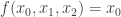
Consider the Boolean function  given by
  .
.
sage: V = GF(2)^4
sage: f = lambda x: x[0]*x[1]+x[2]*x[3]
sage: CartesianProduct(range(16), range(16))
Cartesian product of [0, 1, 2, 3, 4, 5, 6, 7, 8, 9, 10, 11, 12, 13, 14, 15],
                     [0, 1, 2, 3, 4, 5, 6, 7, 8, 9, 10, 11, 12, 13, 14, 15]
sage: C = CartesianProduct(range(16), range(16))
sage: Vlist = V.list()
sage: E = [(x[0],x[1]) for x in C if f(Vlist[x[0]]+Vlist[x[1]])==1]
sage: len(E)
96
sage: E = Set([Set(s) for s in E])
sage: E = [tuple(s) for s in E]
sage: Gamma = Graph(E)
sage: Gamma
Graph on 16 vertices
sage: VG = Gamma.vertices()
sage: L1 = []
sage: L2 = []
sage: for v1 in VG:
....:         for v2 in VG:
....:             N1 = Gamma.neighbors(v1)
....:         N2 = Gamma.neighbors(v2)
....:         if v1 in N2:
....:                 L1 = L1+[len([x for x in N1 if x in N2])]
....:         if not(v1 in N2) and v1!=v2:
....:                 L2 = L2+[len([x for x in N1 if x in N2])]
....:
....:
sage: L1; L2
[2, 2, 2, 2, 2, 2, 2, 2, 2, 2, 2, 2, 2, 2, 2, 2, 2, 2, 2, 2,
 2, 2, 2, 2, 2, 2, 2, 2, 2, 2, 2, 2, 2, 2, 2, 2, 2, 2, 2, 2,
 2, 2, 2, 2, 2, 2, 2, 2, 2, 2, 2, 2, 2, 2, 2, 2, 2, 2, 2, 2,
 2, 2, 2, 2, 2, 2, 2, 2, 2, 2, 2, 2, 2, 2, 2, 2, 2, 2, 2, 2,
 2, 2, 2, 2, 2, 2, 2, 2, 2, 2, 2, 2, 2, 2, 2, 2]
[2, 2, 2, 2, 2, 2, 2, 2, 2, 2, 2, 2, 2, 2, 2, 2, 2, 2, 2, 2,
 2, 2, 2, 2, 2, 2, 2, 2, 2, 2, 2, 2, 2, 2, 2, 2, 2, 2, 2, 2,
 2, 2, 2, 2, 2, 2, 2, 2, 2, 2, 2, 2, 2, 2, 2, 2, 2, 2, 2, 2,
 2, 2, 2, 2, 2, 2, 2, 2, 2, 2, 2, 2, 2, 2, 2, 2, 2, 2, 2, 2,
 2, 2, 2, 2, 2, 2, 2, 2, 2, 2, 2, 2, 2, 2, 2, 2, 2, 2, 2, 2,
 2, 2, 2, 2, 2, 2, 2, 2, 2, 2, 2, 2, 2, 2, 2, 2, 2, 2, 2, 2,
 2, 2, 2, 2, 2, 2, 2, 2, 2, 2, 2, 2, 2, 2, 2, 2, 2, 2, 2, 2,
 2, 2, 2, 2]
This implies the graph is strongly regular with d=e=2.
sage: Gamma.spectrum()
[6, 2, 2, 2, 2, 2, 2, -2, -2, -2, -2, -2, -2, -2, -2, -2]
sage: [walsh_transform(f, a) for a in V]
[4, 4, 4, -4, 4, 4, 4, -4, 4, 4, 4, -4, -4, -4, -4, 4]
sage: Omega_f = [v for v in V if f(v)==1]
sage: len(Omega_f)
6
sage: Gamma.is_bipartite()
False
sage: Gamma.is_hamiltonian()
True
sage: Gamma.is_planar()
False
sage: Gamma.is_regular()
True
sage: Gamma.is_eulerian()
True
sage: Gamma.is_connected()
True
sage: Gamma.is_triangle_free()
False
sage: Gamma.diameter()
2
sage: Gamma.degree_sequence()
[6, 6, 6, 6, 6, 6, 6, 6, 6, 6, 6, 6, 6, 6, 6, 6]
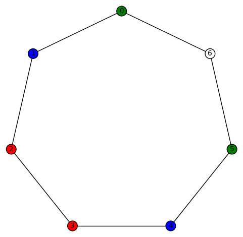
sage: show(Gamma)
# bent-fcns-cayley-graphs1.png
Here is the picture of the graph:

sage: H = matrix(QQ, 16, 16, [(-1)^(Vlist[x[0]]).dot_product(Vlist[x[1]]) for x in C])
sage: H
[ 1  1  1  1  1  1  1  1  1  1  1  1  1  1  1  1]
[ 1 -1  1 -1  1 -1  1 -1  1 -1  1 -1  1 -1  1 -1]
[ 1  1 -1 -1  1  1 -1 -1  1  1 -1 -1  1  1 -1 -1]
[ 1 -1 -1  1  1 -1 -1  1  1 -1 -1  1  1 -1 -1  1]
[ 1  1  1  1 -1 -1 -1 -1  1  1  1  1 -1 -1 -1 -1]
[ 1 -1  1 -1 -1  1 -1  1  1 -1  1 -1 -1  1 -1  1]
[ 1  1 -1 -1 -1 -1  1  1  1  1 -1 -1 -1 -1  1  1]
[ 1 -1 -1  1 -1  1  1 -1  1 -1 -1  1 -1  1  1 -1]
[ 1  1  1  1  1  1  1  1 -1 -1 -1 -1 -1 -1 -1 -1]
[ 1 -1  1 -1  1 -1  1 -1 -1  1 -1  1 -1  1 -1  1]
[ 1  1 -1 -1  1  1 -1 -1 -1 -1  1  1 -1 -1  1  1]
[ 1 -1 -1  1  1 -1 -1  1 -1  1  1 -1 -1  1  1 -1]
[ 1  1  1  1 -1 -1 -1 -1 -1 -1 -1 -1  1  1  1  1]
[ 1 -1  1 -1 -1  1 -1  1 -1  1 -1  1  1 -1  1 -1]
[ 1  1 -1 -1 -1 -1  1  1 -1 -1  1  1  1  1 -1 -1]
[ 1 -1 -1  1 -1  1  1 -1 -1  1  1 -1  1 -1 -1  1]
sage: flist = vector(QQ, [int(f(v)) for v in V])
sage: H*flist
(6, -2, -2, 2, -2, -2, -2, 2, -2, -2, -2, 2, 2, 2, 2, -2)
sage: A = matrix(QQ, 16, 16, [f(Vlist[x[0]]+Vlist[x[1]]) for x in C])
sage: A.eigenvalues()
[6, 2, 2, 2, 2, 2, 2, -2, -2, -2, -2, -2, -2, -2, -2, -2]
Here is another example:  given by
  .
.
sage: V = GF(2)^3
sage: f = lambda x: x[0]*x[1]+x[2]
sage: Omega_f = [v for v in V if f(v)==1]
sage: len(Omega_f)
4
sage: C = CartesianProduct(range(8), range(8))
sage: Vlist = V.list()
sage: E = [(x[0],x[1]) for x in C if f(Vlist[x[0]]+Vlist[x[1]])==1]
sage: E = Set([Set(s) for s in E])
sage: E = [tuple(s) for s in E]
sage: Gamma = Graph(E)
sage: Gamma
Graph on 8 vertices
sage:
sage: VG = Gamma.vertices()
sage: L1 = []
sage: L2 = []
sage: for v1 in VG:
....:         for v2 in VG:
....:             N1 = Gamma.neighbors(v1)
....:         N2 = Gamma.neighbors(v2)
....:         if v1 in N2:
....:                 L1 = L1+[len([x for x in N1 if x in N2])]
....:         if not(v1 in N2) and v1!=v2:
....:                 L2 = L2+[len([x for x in N1 if x in N2])]
....:
sage: L1; L2
[2, 0, 2, 2, 2, 2, 0, 2, 2, 2, 0, 2, 2, 2, 2, 0, 0, 2, 2, 2, 2, 0, 2, 2, 2, 0, 2, 2, 2, 2, 0, 2]
[2, 2, 2, 2, 2, 2, 2, 2, 2, 2, 2, 2, 2, 2, 2, 2, 2, 2, 2, 2, 2, 2, 2, 2]
This implies that the graph is not strongly regular, therefore f is not bent.
sage: Gamma.spectrum()
[4, 2, 0, 0, 0, -2, -2, -2]
sage:
sage: Gamma.is_bipartite()
False
sage: Gamma.is_hamiltonian()
True
sage: Gamma.is_planar()
False
sage: Gamma.is_regular()
True
sage: Gamma.is_eulerian()
True
sage: Gamma.is_connected()
True
sage: Gamma.is_triangle_free()
False
sage: Gamma.diameter()
2
sage: Gamma.degree_sequence()
[4, 4, 4, 4, 4, 4, 4, 4]
sage: H = matrix(QQ, 8, 8, [(-1)^(Vlist[x[0]]).dot_product(Vlist[x[1]]) for x in C])
sage: H
[ 1 1 1 1 1 1 1 1]
[ 1 -1 1 -1 1 -1 1 -1]
[ 1 1 -1 -1 1 1 -1 -1]
[ 1 -1 -1 1 1 -1 -1 1]
[ 1 1 1 1 -1 -1 -1 -1]
[ 1 -1 1 -1 -1 1 -1 1]
[ 1 1 -1 -1 -1 -1 1 1]
[ 1 -1 -1 1 -1 1 1 -1]
sage: flist = vector(QQ, [int(f(v)) for v in V])
sage: H*flist
(4, 0, 0, 0, -2, -2, -2, 2)
sage: Gamma.spectrum()
[4, 2, 0, 0, 0, -2, -2, -2]
sage: A = matrix(QQ, 8, 8, [f(Vlist[x[0]]+Vlist[x[1]]) for x in C])
sage: A.eigenvalues()
[4, 2, 0, 0, 0, -2, -2, -2]
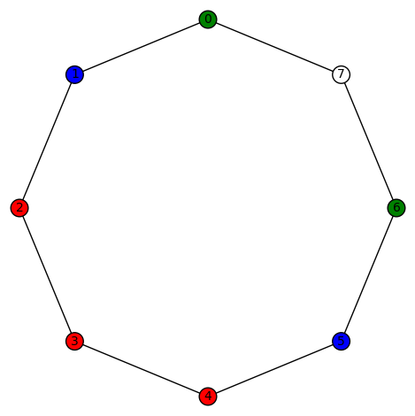
sage: show(Gamma)
# bent-fcns-cayley-graphs2.png
Here is the picture:

REFERENCES:
[1] Pantelimon Stanica, Graph eigenvalues and Walsh spectrum of Boolean functions, INTEGERS 7(2) (2007), #A32.
[2] Anna Bernasconi, Mathematical techniques for the analysis of Boolean functions, Ph. D. dissertation TD-2/98, Universit di Pisa-Udine, 1998.
[3] Anna Bernasconi and Bruno Codenotti, Spectral Analysis of Boolean Functions as a Graph Eigenvalue Problem, IEEE TRANSACTIONS ON COMPUTERS, VOL. 48, NO. 3, MARCH 1999.
[4] A. Bernasconi, B. Codenotti, J.M. VanderKam. A Characterization of Bent Functions in terms of Strongly Regular Graphs, IEEE Transactions on Computers, 50:9 (2001), 984-985.
[5] Michel Mitton, Minimal polynomial of Cayley graph adjacency matrix for Boolean functions, preprint, 2007.
[6] ——, On the Walsh-Fourier analysis of Boolean functions, preprint, 2006.


 to be
to be
 be a harmonic morphism from a graph
  to a graph
  . Then
![{\rm genus}(\Gamma_2)-1 = {\rm deg}(\phi)({\rm genus}(\Gamma_1)-1)+\sum_{x\in V_2} [m_\phi(x)+\frac{1}{2}\nu_\phi(x)-1].](https://s0.wp.com/latex.php?latex=%7B%5Crm+genus%7D%28%5CGamma_2%29-1+%3D+%7B%5Crm+deg%7D%28%5Cphi%29%28%7B%5Crm+genus%7D%28%5CGamma_1%29-1%29%2B%5Csum_%7Bx%5Cin+V_2%7D+%5Bm_%5Cphi%28x%29%2B%5Cfrac%7B1%7D%7B2%7D%5Cnu_%5Cphi%28x%29-1%5D.&bg=ffffff&fg=323232&s=0&c=20201002)
 denotes the horizontal multiplicity and
  denotes the vertical multiplicity.
 -regular and
  -regular.
 be a non-trivial harmonic morphism from a connected
 .
.
 is a harmonic morphism. Let
  be adjacent vertices of
  . Then either (a)
  and
and  “collapses” the edge (vertical)
  or (b)
  and the vertices
  and
and  are adjacent in
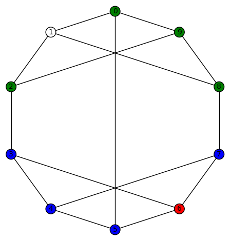
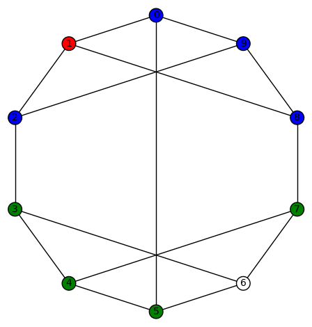
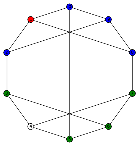
  . In the particular case of this post (ie, the case of
  the white vertex is not adjacent to the blue or red vertex, none of the harmonic colored graphs below can have a white vertex adjacent to a blue or red vertex.
 as the domain in this post. However, before we get to examples (obtained by using
  be a harmonic morphism from a graph
  vertices to the path graph having
  vertices. Let
  be the coloring map (identified with an n-tuple whose coordinates are in
  ). Associated to f is a partition
 ![\Pi_f=[n_0,\dots,n_{k-1}]](https://s0.wp.com/latex.php?latex=%5CPi_f%3D%5Bn_0%2C%5Cdots%2Cn_%7Bk-1%7D%5D&bg=ffffff&fg=323232&s=0&c=20201002) of n (here
of n (here ![[...]](https://s0.wp.com/latex.php?latex=%5B...%5D&bg=ffffff&fg=323232&s=0&c=20201002) is a multi-set, so repetition is allowed but the ordering is unimportant):
is a multi-set, so repetition is allowed but the ordering is unimportant):  , where
  is the number of times j occurs in f. We call this the partition invariant of the harmonic morphism.
  ,
,  , with associated
 whose corresponding partitions agree,
  then we say
  and
and  are partition equivalent.
 examples!
 , so we start with
  . We indicate a harmonic morphism by a vertex coloring. An example of a harmonic morphism can be described in the plot below as follows:
  sends the red vertices in
  , plus that induced by
  and all of its cyclic permutations (4+6=10). This set of 6 permutations is closed under the automorphism of
 and all of its cyclic permutations (4+7=11). This set of 7 permutations is not closed under the automorphism of
  and all 7 of its cyclic permutations (total = 7+11 = 18).
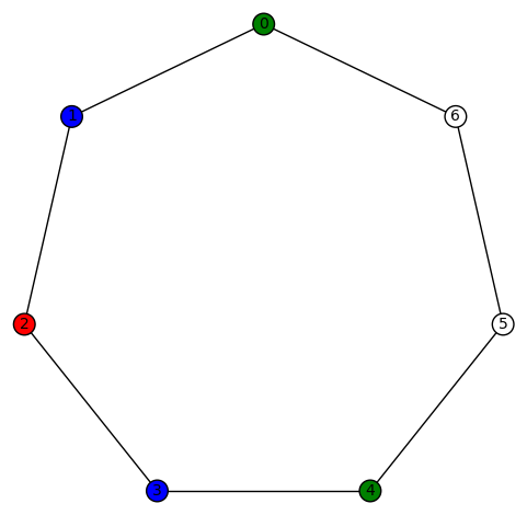
 and all of its cyclic permutations (4+8=12). This set of 8 permutations is not closed under the automorphism of
  and all of its cyclic permutations (12+8=20). In addition, there is
  and all of its cyclic permutations (20+8 = 28). The latter set of 8 cyclic permutations of
  is closed under the transposition (0,3)(1,2) (total = 28).

 and all of its cyclic permutations (4+9=13). This set of 9 permutations is not closed under the automorphism of
  and all 9 of its cyclic permutations (9+13 = 22). This set of 9 permutations is not closed under the automorphism of
  and all 9 of its cyclic permutations (9+22 = 31). This set of 9 permutations is not closed under the automorphism of
  and all 9 of its cyclic permutations (total = 9+31 = 40).


 is the graph whose SageMath command is


 then, instead of showing a graph, I’ll list the edges (of course, the vertices are 0,1,…,11) and the SageMath command for it.
 , where
  .
. .
. .
. .
. .
. .
. .
. and
and  then this is a list of length
  consisting of elements taken from the
  vertices in
  .
. and let
  .
.

 by
by of a graph
  to be a subgraph of
  is called harmonic if for all vertices
  , the quantity
 in
in  .
. , we may identify a Boolean function

 , let
, let  denote the set of complements
  , for
, for  , and let
  denote the complementary Boolean function. Note that
 denotes the complement of
  in
in 
 is even (resp., odd). We may identify a vector in
  Let
Let
 ).
). denote the $2^n\times 2^n$ Hadamard matrix defined by
  , for each
  such that
  . Inductively, these can be defined by
 whose
whose  th component is
 as the column vector where the
  th component is
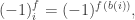
 .
.
 . It is even because
 be the Cayley graph of
 so
so  has no loops. In this case,
  -regular graph having
  connected components, where
 , the set of neighbors
  of
of 
 be the
  adjacency matrix of


 of the adjacency matrix
  ) to the Walsh-Hadamard transform
  . Note that
  where
where  . She discovered the relationship
 be the binary Hamming [7,4,3] code defined by the generator matrix
 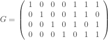 and check matrix
 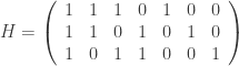 . In other words, this code is the row space of G and the kernel of H. We can enter these into Sage as follows:
 defined by
  . Using this map, the codewords are easy to describe and enumerate:
 .
. . This must be a codeword (no lies) or differ from a codeword by exactly one bit (1 lie). In either case, you can find n by decoding this vector.
 .
. in region i of the Venn diagram.


 , for some unknown
  . We solve for this unknown using the check vertex equation
  . The decoded codeword is
 . In this case, we know the vertices 9 and 10 fail, so
  . We solve using

 . By majority vote, we get
  .
. 

 be a weighted digraph having
  denote its
 adjacency matrix. We identify the vertices with the set
  .
. n-1 in row i and column j equals the length of a shortest path from vertex i to vertex j in G. (Here A
 is equal to A
 This verifies an example given in chapter 1 of the book by Maclagan and Sturmfels,
  be a weighted digraph having
  denote its
  adjacency matrix. We identify the vertices with the set
  , is defined with the operations as follows:
  ,
,  . The ordinary product of two
  operations (roughly the same number of additions and multiplications). The tropical product of two
  , where M is the complexity of computing the (tropical) product of two
  time. However, the implied “big-O” constant is so large that the algorithm is not practical. Strassen’s algorithm can multiply two
  time.
time.  , using Strassen’s algorithm. This is better than the
You must be logged in to post a comment.