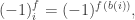
Boolean functions from the graph-theoretic perspective

Posted on 2012/09/08 by wdjoyner

This is a very short introductory survey of graph-theoretic properties of Boolean functions.

I don’t know who first studied Boolean functions for their own sake. However, the study of Boolean functions from the graph-theoretic perspective originated in Anna Bernasconi‘s thesis. More detailed presentation of the material can be found in various places. For example, Bernasconi’s thesis (e.g., see [BC]), the nice paper by P. Stanica (e.g., see [S], or his book with T. Cusick), or even my paper with Celerier, Melles and Phillips (e.g., see [CJMP], from which much of this material is literally copied).

For a given positive integer $n$ , we may identify a Boolean function

$f:GF(2)^n\to GF(2),$
with its support

$\Omega_f = \{x\in GF(2)^n\ |\ f(x)=1\}.$

For each $S\subset GF(2)^n$ , let $\overline{S}$ denote the set of complements $\overline{x}=x+(1,\dots,1)\in GF(2)^n$ , for $x\in S$ , and let $\overline{f}=f+1$ denote the complementary Boolean function. Note that

$\Omega_f^c=\Omega_{\overline{f}},$

where $S^c$ denotes the complement of $S$ in $GF(2)^n$ . Let

$\omega=\omega_f=|\Omega_f|$

denote the cardinality of the support. We call a Boolean function even (resp., odd) if $\omega_f$ is even (resp., odd). We may identify a vector in $GF(2)^n$ with its support, or, if it is more convenient, with the corresponding integer in $\{0,1, \dots, 2^n-1\}.$ Let

$b:\{0,1, \dots, 2^n-1\} \to GF(2)^n$

be the binary representation ordered with least significant bit last (so that, for example, $b(1)=(0,\dots, 0, 1)\in GF(2)^n$ ).

Let $H_n$ denote the $2^n\times 2^n$ Hadamard matrix defined by $(H_n)_{i,j} = (-1)^{b(i)\cdot b(j)}$ , for each $i,j$ such that $0\leq i,j\leq n-1$ . Inductively, these can be defined by

$H_1 = \left( \begin{array}{cc} 1 & 1\\ 1 & -1 \\ \end{array} \right), \ \ \ \ \ \ H_n = \left( \begin{array}{cc} H_{n-1} & H_{n-1}\\ H_{n-1} & -H_{n-1} \\ \end{array} \right), \ \ \ \ \ n>1.$
The Walsh-Hadamard transform of $f$ is defined to be the vector in ${\mathbb{R}}^{2^n}$ whose $k$ th component is

$({\mathcal{H}} f)(k) = \sum_{i \in \{0,1,\ldots,2^n-1\}}(-1)^{b(i) \cdot b(k) + f(b(i))} = (H_n (-1)^f)_k,$

where we define $(-1)^f$ as the column vector where the $i$ th component is

$(-1)^f_i = (-1)^{f(b(i))},$

for $i = 0,\ldots,2^n-1$ .

Example
A Boolean function of three variables cannot be bent. Let $f$ be defined by:

$\begin{array}{c|cccccccc} x_2 & 0 & 0 & 0 & 0 & 1 & 1 & 1 & 1 \\ x_1 & 0 & 0 & 1 & 1 & 0 & 0 & 1 & 1 \\ x_0 & 0 & 1 & 0 & 1 & 0 & 1 & 0 & 1 \\ \hline (-1)^f & 1 & -1 & 1 & -1 & 1 & -1 & 1 & -1 \\ {\mathcal{H}}f & 0 & 8 & 0 & 0 & 0 & 0 & 0 & 0 \\ \end{array}$
This is simply the function $f(x_0,x_1,x_2)=x_0$ . It is even because

$\Omega_f = \{ (0,0,1), (0,1,1), (1,0,1), (1,1,1) \},\ \mbox{ so } \ \omega = 4.$

Here is some Sage code verifying this:

sage: from sage.crypto.boolean_function import *
sage: f = BooleanFunction([0,1,0,1,0,1,0,1])
sage: f.algebraic_normal_form()
x0
sage: f.walsh_hadamard_transform()
(0, -8, 0, 0, 0, 0, 0, 0)

(The Sage method walsh_hadamard_transform is off by a sign from the definition we gave.) We will return to this example later.

Let $X=(V,E)$ be the Cayley graph of $f$ :

$V = GF(2)^n,\ \ \ \ E = \{(v,w)\in V\times V\ |\ f(v+w)=1\}.$
We shall assume throughout and without further mention that $f(0)\not=1,$ so $X$ has no loops. In this case, $X$ is an $\omega$ -regular graph having $r$ connected components, where

$r = |GF(2)^n/{\rm Span}(\Omega_f)|.$

For each vertex $v\in V$ , the set of neighbors $N(v)$ of $v$ is given by

$N(v)=v+\Omega_f,$

where $v$ is regarded as a vector and the addition is induced by the usual vector addition in $GF(2)^n$ . Let $A = (A_{ij})$ be the $2^n\times 2^n$ adjacency matrix of $X$ , so

$A_{ij} = f(b(i)+b(j)), \ \ \ \ \ 0\leq i,j\leq 2^n-1.$

Example:
Returning to the previous example, we construct its Cayley graph.

First, attach afsr.sage from [C] in your Sage session.

     sage: flist = [0,1,0,1,0,1,0,1]
     sage: V = GF(2)ˆ3
     sage: Vlist = V.list()
     sage: f = lambda x: GF(2)(flist[Vlist.index(x)])
     sage: X = boolean_cayley_graph(f, 3)
     sage: X.adjacency_matrix()
     [0 1 0 1 0 1 0 1]
     [1 0 1 0 1 0 1 0]
     [0 1 0 1 0 1 0 1]
     [1 0 1 0 1 0 1 0]
     [0 1 0 1 0 1 0 1]
     [1 0 1 0 1 0 1 0]
     [0 1 0 1 0 1 0 1]
     [1 0 1 0 1 0 1 0]
     sage: X.spectrum()
     [4, 0, 0, 0, 0, 0, 0, -4]
     sage: X.show(layout="circular")

In her thesis, Bernasconi found a relationship between the spectrum of the Cayley graph $X$ ,

${\rm Spectrum}(X) = \{\lambda_k\ |\ 0\leq k\leq 2^n-1\},$

(the eigenvalues $\lambda_k$ of the adjacency matrix $A$ ) to the Walsh-Hadamard transform $\mathcal H f = H_n (-1)^f$ . Note that $f$ and $(-1)^f$ are related by the equation $f=\frac 1 2 (e - (-1)^f),$ where $e=(1,1,...,1)$ . She discovered the relationship

$\lambda_k = \frac 1 2 (H_n e - \mathcal H f)_k$

between the spectrum of the Cayley graph $X$ of a Boolean function and the values of the Walsh-Hadamard transform of the function. Therefore, the spectrum of $X$ , is explicitly computable as an expression in terms of $f$ .

References:

[BC] A. Bernasconi and B. Codenotti, Spectral analysis of Boolean functions as a graph eigenvalue problem, IEEE Trans. Computers 48(1999)345-351.

[CJMP] Charles Celerier, David Joyner, Caroline Melles, David Phillips, On the Hadamard transform of monotone Boolean functions, Tbilisi Mathematical Journal, Volume 5, Issue 2 (2012), 19-35.

[S] P. Stanica, Graph eigenvalues and Walsh spectrum of Boolean functions, Integers 7(2007)\# A32, 12 pages.

Here’s an excellent video of Pante Stanica on interesting applications of Boolean functions to cryptography (30 minutes):

Some remarks on monotone Boolean functions

Posted on 2012/09/01 by wdjoyner

This post summarizes some joint research with Charles Celerier, Caroline Melles, and David Phillips.

Let $f:GF(2)^n \to GF(2)$ be a Boolean function. (We identify $GF(2)$ with either the real numbers $\{0,1\}$ or the binary field ${\mathbb{Z}}/2{\mathbb{Z}}$ . Hopefully, the context makes it clear which one is used.)

Define a partial order $\leq$ on $GF(2)^n$ as follows: for each $v,w\in GF(2)^n$ , we say $v\leq w$ whenever we have $v_1 \leq w_1$ , $v_2 \leq w_2$ , …, $v_n \leq w_n$ . A Boolean function is called monotone (increasing) if whenever we have $v\leq w$ then we also have $f(v) \leq f(w)$ .

Note that if $f$ and $g$ are monotone then (a) $f+g+fg$ is also monotone, and (b) $\overline{\Omega_f}\cap \overline{\Omega_g}=\overline{\Omega_{fg}}$ . (Overline means bit-wise complement.)

Definition:
Let $f:GF(2)^n \to GF(2)$ be any monotone function. We say that $\Gamma\subset GF(2)^n$ is the least support of $f$ if $\Gamma$ consists of all vectors in $\Omega_f$ which are smallest in the partial ordering $\leq$ on $GF(2)^n$ . We say a subset $S$ of $GF(2)^n$ is admissible if for all $x,y\in S$ , ${\rm supp}(x)\not\subset {\rm supp}(y)$ and ${\rm supp}(y)\not\subset {\rm supp}(x)$

Monotone functions on $GF(2)^n$ are in a natural one-to-one correspondence with the collection of admissible sets.

Example:
Here is an example of a monotone function whose least support vectors are given by
$\Gamma =\{ (1,0,0,0), (0,1,1,0), (0,1,0,1), (0,0,1,1) \} \subset GF(2)^n,$
illustrated in the figure below.

The algebraic normal form is $x_0x_1x_2 + x_0x_1x_3 + x_0x_2x_3 + x_1x_2 + x_1x_3 + x_2x_3 + x_0$ .

The following result is due to Charles Celerier.

Theorem:
Let $f$ be a monotone function whose least support vectors are given by $\Gamma \subset GF(2)^n$ . Then
$f(x) = 1+\prod_{v\in\Gamma} (x^v+1).$

The following example is due to Caroline Melles.

Example:
Let $f$ be the monotone function whose least support is
$\Gamma = \{ (1,1,1,1,0,0),(1,1,0,0,1,1),(0,0,1,1,1,1)\}.$
Using the Theorem above, we obtain the compact algebraic form
$f(x_0,x_1,x_2,x_3,x_4,x_5) = x_0x_1x_2x_3 + x_0x_1x_4x_5 + x_2x_3x_4x_5 .$
This function is monotone yet has no vanishing Walsh-Hadamard transform values. To see this, we attach the file afsr.sage available from Celerier (https://github.com/celerier/oslo/), then run the following commands.

sage: V = GF(2)^(6)
sage: L = [V([1,1,0,0,1,1]),V([0,0,1,1,1,1]), V([1,1,1,1,0,0])]
sage: f = monotone_from_support(L)
sage: is_monotone(f)
True

These commands simply construct a Boolean function $f$ whose least support are the vectors in L. Next, we compute the Walsh-Hadamard transform of this using both the method built into Sage’s sage.crypto module, and the function in afsr.sage.

sage: f.walsh_hadamard_transform()
(-44, -12, -12, 12, -12, 4, 4, -4, -12, 4, 4, -4, 12, -4, -4, 4, -12, 4, 4, -4, 4, 4, 4, -4, 4, 4, 4, -4, -4, 
 -4, -4, 4, -12, 4, 4, -4, 4, 4, 4, -4, 4, 4, 4, -4, -4, -4, -4, 4, 12, -4, -4, 4, -4, -4, -4, 4, -4, -4, -4, 4, 4, 4, 4, -4)
sage: f.algebraic_normal_form()
x0*x1*x2*x3 + x0*x1*x4*x5 + x2*x3*x4*x5
sage: x0,x1,x2,x3,x4,x5 = var("x0,x1,x2,x3,x4,x5")
sage: g = x0*x1*x2*x3 + x0*x1*x4*x5 + x2*x3*x4*x5
sage: Omega = [v for v in V if g(x0=v[0], x1=v[1], x2=v[2], x3=v[3],
     x4=v[4], x5=v[5])0]
sage: len(Omega)
10
sage: g = lambda x: x[0]*x[1]*x[2]*x[3] + x[0]*x[1]*x[4]*x[5] + x[2]*x[3]*x[4]*x[5]
sage: [walsh_transform(g,a) for a in V]
[44, 12, 12, -12, 12, -4, -4, 4, 12, -4, -4, 4, -12, 4, 4, -4, 12, -4, -4, 4, -4, -4, -4, 4, -4, -4, -4, 4, 4, 
 4, 4, -4, 12, -4, -4, 4, -4, -4, -4, 4, -4, -4, -4, 4, 4, 4, 4, -4, -12, 4, 4, -4, 4, 4, 4, -4, 4, 4, 4, -4, -4, -4, -4, 4]

(Note: the Walsh transform method in the BooleanFunction class in Sage differs by a sign from the standard definition.) This verifies that there are no values of the Walsh-Hadamard transform which are $0$ .

More details can be found in the paper listed here. I end with two questions (which I think should be answered “no”).

Question: Are there any monotone functions $f$ of $n$ variables having no free variables of degree $\leq n/2$ ?

Question: Are there any monotone functions $f$ of most than two variables which are bent?

Applications of graphs to Boolean functions

Posted on 2012/02/16 by wdjoyner

Let f be a Boolean function on $GF(2)^n$ . The Cayley graph of f is defined to be the graph

$\Gamma_f = (GF(2)^n, E_f )$ ,

whose vertex set is $GF(2)^n$ and the set of edges is defined by

$E_f =\{ (u,v) \in GF(2)^n \times GF(2)^n \ |\ f(u+v)=1\}$ .

The adjacency matrix $A_f$ is the matrix whose entries are

$A_{i,j} = f(b(i) + b(j))$ ,

where b(k) is the binary representation of the integer k.
Note $\Gamma_f$ is a regular graph of degree wt(f), where wt denotes the Hamming weight of f when regarded as a vector of values (of length $2^n$ ).

Recall that, given a graph $\Gamma$ and its adjacency matrix A, the spectrum Spec( $\Gamma$ ) is the multi-set of eigenvalues of A.

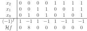
The Walsh transform of a Boolean function f is an integer-valued function over $GF(2)^n$ that can be defined as

$W_f(u) = \sum_{x in GF(2)^n} (-1)^{f(x)+ \langle u,x\rangle}.$
A Boolean function f is bent if $|W_f(a)| = 2^{n/2}$ (this only makes sense if n is even). The Hadamard transform of a integer-valued function f is an integer-valued function over $GF(2)^n$ that can be defined as

$H_f(u) = \sum_{x in GF(2)^n} f(x)(-1)^{\langle u,x\rangle}.$
It turns out that the spectrum of $\Gamma_f$ is equal to the Hadamard transform of f when regarded as a vector of (integer) 0,1-values. (This nice fact seems to have first appeared in [2], [3].)

A graph is regular of degree r (or r-regular) if every vertex has degree r (number of edges incident to it).   We say that an r-regular graph $\Gamma$ is a strongly regular graph with parameters (v, r, d, e) (for nonnegative integers e, d) provided, for all vertices u, v the number of vertices adjacent to both u, v is equal to

          e, if u, v are adjacent,
          d, if u, v are nonadjacent.

It turns out tht f is bent iff $\Gamma_f$ is strongly regular and e = d (see [3] and [4]).

The following Sage computations illustrate these and other theorems in [1], [2], [3], [4].

Consider the Boolean function $f: GF(2)^4 \to GF(2)$ given by $f(x_0,x_1,x_2) = x_0x_1+x_2x_3$ .

sage: V = GF(2)^4
sage: f = lambda x: x[0]*x[1]+x[2]*x[3]
sage: CartesianProduct(range(16), range(16))
Cartesian product of [0, 1, 2, 3, 4, 5, 6, 7, 8, 9, 10, 11, 12, 13, 14, 15], 
                     [0, 1, 2, 3, 4, 5, 6, 7, 8, 9, 10, 11, 12, 13, 14, 15]
sage: C = CartesianProduct(range(16), range(16))
sage: Vlist = V.list()                  
sage: E = [(x[0],x[1]) for x in C if f(Vlist[x[0]]+Vlist[x[1]])==1]
sage: len(E)
96
sage: E = Set([Set(s) for s in E])
sage: E = [tuple(s) for s in E] 
sage: Gamma = Graph(E)
sage: Gamma
Graph on 16 vertices
sage: VG = Gamma.vertices()
sage: L1 = []
sage: L2 = []
sage: for v1 in VG:
....:         for v2 in VG:
....:             N1 = Gamma.neighbors(v1)
....:         N2 = Gamma.neighbors(v2)
....:         if v1 in N2:
....:                 L1 = L1+[len([x for x in N1 if x in N2])]
....:         if not(v1 in N2) and v1!=v2:
....:                 L2 = L2+[len([x for x in N1 if x in N2])]
....: 
....: 
sage: L1; L2
[2, 2, 2, 2, 2, 2, 2, 2, 2, 2, 2, 2, 2, 2, 2, 2, 2, 2, 2, 2,
 2, 2, 2, 2, 2, 2, 2, 2, 2, 2, 2, 2, 2, 2, 2, 2, 2, 2, 2, 2,
 2, 2, 2, 2, 2, 2, 2, 2, 2, 2, 2, 2, 2, 2, 2, 2, 2, 2, 2, 2,
 2, 2, 2, 2, 2, 2, 2, 2, 2, 2, 2, 2, 2, 2, 2, 2, 2, 2, 2, 2,
 2, 2, 2, 2, 2, 2, 2, 2, 2, 2, 2, 2, 2, 2, 2, 2]
[2, 2, 2, 2, 2, 2, 2, 2, 2, 2, 2, 2, 2, 2, 2, 2, 2, 2, 2, 2,
 2, 2, 2, 2, 2, 2, 2, 2, 2, 2, 2, 2, 2, 2, 2, 2, 2, 2, 2, 2,
 2, 2, 2, 2, 2, 2, 2, 2, 2, 2, 2, 2, 2, 2, 2, 2, 2, 2, 2, 2,
 2, 2, 2, 2, 2, 2, 2, 2, 2, 2, 2, 2, 2, 2, 2, 2, 2, 2, 2, 2,
 2, 2, 2, 2, 2, 2, 2, 2, 2, 2, 2, 2, 2, 2, 2, 2, 2, 2, 2, 2,
 2, 2, 2, 2, 2, 2, 2, 2, 2, 2, 2, 2, 2, 2, 2, 2, 2, 2, 2, 2,
 2, 2, 2, 2, 2, 2, 2, 2, 2, 2, 2, 2, 2, 2, 2, 2, 2, 2, 2, 2,
 2, 2, 2, 2]

This implies the graph is strongly regular with d=e=2.

sage: Gamma.spectrum()
[6, 2, 2, 2, 2, 2, 2, -2, -2, -2, -2, -2, -2, -2, -2, -2]
sage: [walsh_transform(f, a) for a in V]
[4, 4, 4, -4, 4, 4, 4, -4, 4, 4, 4, -4, -4, -4, -4, 4]
sage: Omega_f = [v for v in V if f(v)==1] 
sage: len(Omega_f)
6
sage: Gamma.is_bipartite()
False
sage: Gamma.is_hamiltonian()
True
sage: Gamma.is_planar()     
False
sage: Gamma.is_regular()
True
sage: Gamma.is_eulerian()
True
sage: Gamma.is_connected()
True
sage: Gamma.is_triangle_free()
False
sage: Gamma.diameter()
2
sage: Gamma.degree_sequence()
[6, 6, 6, 6, 6, 6, 6, 6, 6, 6, 6, 6, 6, 6, 6, 6]
sage: show(Gamma)
# bent-fcns-cayley-graphs1.png

Here is the picture of the graph:

sage: H = matrix(QQ, 16, 16, [(-1)^(Vlist[x[0]]).dot_product(Vlist[x[1]]) for x in C])
sage: H
[ 1  1  1  1  1  1  1  1  1  1  1  1  1  1  1  1]
[ 1 -1  1 -1  1 -1  1 -1  1 -1  1 -1  1 -1  1 -1]
[ 1  1 -1 -1  1  1 -1 -1  1  1 -1 -1  1  1 -1 -1]
[ 1 -1 -1  1  1 -1 -1  1  1 -1 -1  1  1 -1 -1  1]
[ 1  1  1  1 -1 -1 -1 -1  1  1  1  1 -1 -1 -1 -1]
[ 1 -1  1 -1 -1  1 -1  1  1 -1  1 -1 -1  1 -1  1]
[ 1  1 -1 -1 -1 -1  1  1  1  1 -1 -1 -1 -1  1  1]
[ 1 -1 -1  1 -1  1  1 -1  1 -1 -1  1 -1  1  1 -1]
[ 1  1  1  1  1  1  1  1 -1 -1 -1 -1 -1 -1 -1 -1]
[ 1 -1  1 -1  1 -1  1 -1 -1  1 -1  1 -1  1 -1  1]
[ 1  1 -1 -1  1  1 -1 -1 -1 -1  1  1 -1 -1  1  1]
[ 1 -1 -1  1  1 -1 -1  1 -1  1  1 -1 -1  1  1 -1]
[ 1  1  1  1 -1 -1 -1 -1 -1 -1 -1 -1  1  1  1  1]
[ 1 -1  1 -1 -1  1 -1  1 -1  1 -1  1  1 -1  1 -1]
[ 1  1 -1 -1 -1 -1  1  1 -1 -1  1  1  1  1 -1 -1]
[ 1 -1 -1  1 -1  1  1 -1 -1  1  1 -1  1 -1 -1  1]
sage: flist = vector(QQ, [int(f(v)) for v in V])
sage: H*flist  
(6, -2, -2, 2, -2, -2, -2, 2, -2, -2, -2, 2, 2, 2, 2, -2)
sage: A = matrix(QQ, 16, 16, [f(Vlist[x[0]]+Vlist[x[1]]) for x in C])
sage: A.eigenvalues()
[6, 2, 2, 2, 2, 2, 2, -2, -2, -2, -2, -2, -2, -2, -2, -2]

Here is another example: $f: GF(2)^3 \to GF(2)$ given by $f(x_0,x_1,x_2) = x_0x_1+x_2$ .

sage: V = GF(2)^3
sage: f = lambda x: x[0]*x[1]+x[2]
sage: Omega_f = [v for v in V if f(v)==1] 
sage: len(Omega_f)
4
sage: C = CartesianProduct(range(8), range(8))
sage: Vlist = V.list()    
sage: E = [(x[0],x[1]) for x in C if f(Vlist[x[0]]+Vlist[x[1]])==1]
sage: E = Set([Set(s) for s in E])
sage: E = [tuple(s) for s in E] 
sage: Gamma = Graph(E)
sage: Gamma
Graph on 8 vertices
sage: 
sage: VG = Gamma.vertices()
sage: L1 = []
sage: L2 = []
sage: for v1 in VG:
....:         for v2 in VG:
....:             N1 = Gamma.neighbors(v1)
....:         N2 = Gamma.neighbors(v2)
....:         if v1 in N2:
....:                 L1 = L1+[len([x for x in N1 if x in N2])]
....:         if not(v1 in N2) and v1!=v2:
....:                 L2 = L2+[len([x for x in N1 if x in N2])]
....: 
sage: L1; L2
[2, 0, 2, 2, 2, 2, 0, 2, 2, 2, 0, 2, 2, 2, 2, 0, 0, 2, 2, 2, 2, 0, 2, 2, 2, 0, 2, 2, 2, 2, 0, 2]
[2, 2, 2, 2, 2, 2, 2, 2, 2, 2, 2, 2, 2, 2, 2, 2, 2, 2, 2, 2, 2, 2, 2, 2]

This implies that the graph is not strongly regular, therefore f is not bent.

sage: Gamma.spectrum()
[4, 2, 0, 0, 0, -2, -2, -2]
sage: 
sage: Gamma.is_bipartite()
False
sage: Gamma.is_hamiltonian()
True
sage: Gamma.is_planar()     
False
sage: Gamma.is_regular()
True
sage: Gamma.is_eulerian()
True
sage: Gamma.is_connected()
True
sage: Gamma.is_triangle_free()
False
sage: Gamma.diameter()
2
sage: Gamma.degree_sequence()
[4, 4, 4, 4, 4, 4, 4, 4]
sage: H = matrix(QQ, 8, 8, [(-1)^(Vlist[x[0]]).dot_product(Vlist[x[1]]) for x in C])
sage: H
[ 1  1  1  1  1  1  1  1]
[ 1 -1  1 -1  1 -1  1 -1]
[ 1  1 -1 -1  1  1 -1 -1]
[ 1 -1 -1  1  1 -1 -1  1]
[ 1  1  1  1 -1 -1 -1 -1]
[ 1 -1  1 -1 -1  1 -1  1]
[ 1  1 -1 -1 -1 -1  1  1]
[ 1 -1 -1  1 -1  1  1 -1]
sage: flist = vector(QQ, [int(f(v)) for v in V])
sage: H*flist  
(4, 0, 0, 0, -2, -2, -2, 2)
sage: Gamma.spectrum()
[4, 2, 0, 0, 0, -2, -2, -2]
sage: A = matrix(QQ, 8, 8, [f(Vlist[x[0]]+Vlist[x[1]]) for x in C])
sage: A.eigenvalues()
[4, 2, 0, 0, 0, -2, -2, -2]

sage: show(Gamma)
# bent-fcns-cayley-graphs2.png

Here is the picture:

REFERENCES:
[1] Pantelimon Stanica, Graph eigenvalues and Walsh spectrum of Boolean functions, INTEGERS 7(2) (2007), #A32.

[2] Anna Bernasconi, Mathematical techniques for the analysis of Boolean functions, Ph. D. dissertation TD-2/98, Universit di Pisa-Udine, 1998.

[3] Anna Bernasconi and Bruno Codenotti, Spectral Analysis of Boolean Functions as a Graph Eigenvalue Problem, IEEE TRANSACTIONS ON COMPUTERS, VOL. 48, NO. 3, MARCH 1999.

[4] A. Bernasconi, B. Codenotti, J.M. VanderKam. A Characterization of Bent Functions in terms of Strongly Regular Graphs, IEEE Transactions on Computers, 50:9 (2001), 984-985.

[5] Michel Mitton, Minimal polynomial of Cayley graph adjacency matrix for Boolean functions, preprint, 2007.

[6] ——, On the Walsh-Fourier analysis of Boolean functions, preprint, 2006.

M	T	W	T	F	S	S
		1	2	3	4	5
6	7	8	9	10	11	12
13	14	15	16	17	18	19
20	21	22	23	24	25	26
27	28	29	30	31

Yet Another Mathblog

Tag Archives: Boolean functions

Boolean functions from the graph-theoretic perspective

Some remarks on monotone Boolean functions

Applications of graphs to Boolean functions