Boolean functions from the graph-theoretic perspective

This is a very short introductory survey of graph-theoretic properties of Boolean functions.

I don’t know who first studied Boolean functions for their own sake. However, the study of Boolean functions from the graph-theoretic perspective originated in Anna Bernasconi‘s thesis. More detailed presentation of the material can be found in various places. For example, Bernasconi’s thesis (e.g., see [BC]), the nice paper by P. Stanica (e.g., see [S], or his book with T. Cusick), or even my paper with Celerier, Melles and Phillips (e.g., see [CJMP], from which much of this material is literally copied).

For a given positive integer $n$ , we may identify a Boolean function

$f:GF(2)^n\to GF(2),$
with its support

$\Omega_f = \{x\in GF(2)^n\ |\ f(x)=1\}.$

For each $S\subset GF(2)^n$ , let $\overline{S}$ denote the set of complements $\overline{x}=x+(1,\dots,1)\in GF(2)^n$ , for $x\in S$ , and let $\overline{f}=f+1$ denote the complementary Boolean function. Note that

$\Omega_f^c=\Omega_{\overline{f}},$

where $S^c$ denotes the complement of $S$ in $GF(2)^n$ . Let

$\omega=\omega_f=|\Omega_f|$

denote the cardinality of the support. We call a Boolean function even (resp., odd) if $\omega_f$ is even (resp., odd). We may identify a vector in $GF(2)^n$ with its support, or, if it is more convenient, with the corresponding integer in $\{0,1, \dots, 2^n-1\}.$ Let

$b:\{0,1, \dots, 2^n-1\} \to GF(2)^n$

be the binary representation ordered with least significant bit last (so that, for example, $b(1)=(0,\dots, 0, 1)\in GF(2)^n$ ).

Let $H_n$ denote the $2^n\times 2^n$ Hadamard matrix defined by $(H_n)_{i,j} = (-1)^{b(i)\cdot b(j)}$ , for each $i,j$ such that $0\leq i,j\leq n-1$ . Inductively, these can be defined by

$H_1 = \left( \begin{array}{cc} 1 & 1\\ 1 & -1 \\ \end{array} \right), \ \ \ \ \ \ H_n = \left( \begin{array}{cc} H_{n-1} & H_{n-1}\\ H_{n-1} & -H_{n-1} \\ \end{array} \right), \ \ \ \ \ n>1.$
The Walsh-Hadamard transform of $f$ is defined to be the vector in ${\mathbb{R}}^{2^n}$ whose $k$ th component is

$({\mathcal{H}} f)(k) = \sum_{i \in \{0,1,\ldots,2^n-1\}}(-1)^{b(i) \cdot b(k) + f(b(i))} = (H_n (-1)^f)_k,$

where we define $(-1)^f$ as the column vector where the $i$ th component is

$(-1)^f_i = (-1)^{f(b(i))},$

for $i = 0,\ldots,2^n-1$ .

Example
A Boolean function of three variables cannot be bent. Let $f$ be defined by:

$\begin{array}{c|cccccccc} x_2 & 0 & 0 & 0 & 0 & 1 & 1 & 1 & 1 \\ x_1 & 0 & 0 & 1 & 1 & 0 & 0 & 1 & 1 \\ x_0 & 0 & 1 & 0 & 1 & 0 & 1 & 0 & 1 \\ \hline (-1)^f & 1 & -1 & 1 & -1 & 1 & -1 & 1 & -1 \\ {\mathcal{H}}f & 0 & 8 & 0 & 0 & 0 & 0 & 0 & 0 \\ \end{array}$
This is simply the function $f(x_0,x_1,x_2)=x_0$ . It is even because

$\Omega_f = \{ (0,0,1), (0,1,1), (1,0,1), (1,1,1) \},\ \mbox{ so } \ \omega = 4.$

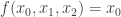
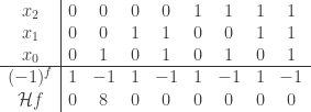
Here is some Sage code verifying this:

sage: from sage.crypto.boolean_function import *
sage: f = BooleanFunction([0,1,0,1,0,1,0,1])
sage: f.algebraic_normal_form()
x0
sage: f.walsh_hadamard_transform()
(0, -8, 0, 0, 0, 0, 0, 0)

(The Sage method walsh_hadamard_transform is off by a sign from the definition we gave.) We will return to this example later.

Let $X=(V,E)$ be the Cayley graph of $f$ :

$V = GF(2)^n,\ \ \ \ E = \{(v,w)\in V\times V\ |\ f(v+w)=1\}.$
We shall assume throughout and without further mention that $f(0)\not=1,$ so $X$ has no loops. In this case, $X$ is an $\omega$ -regular graph having $r$ connected components, where

$r = |GF(2)^n/{\rm Span}(\Omega_f)|.$

For each vertex $v\in V$ , the set of neighbors $N(v)$ of $v$ is given by

$N(v)=v+\Omega_f,$

where $v$ is regarded as a vector and the addition is induced by the usual vector addition in $GF(2)^n$ . Let $A = (A_{ij})$ be the $2^n\times 2^n$ adjacency matrix of $X$ , so

$A_{ij} = f(b(i)+b(j)), \ \ \ \ \ 0\leq i,j\leq 2^n-1.$

Example:
Returning to the previous example, we construct its Cayley graph.

First, attach afsr.sage from [C] in your Sage session.

     sage: flist = [0,1,0,1,0,1,0,1]
     sage: V = GF(2)ˆ3
     sage: Vlist = V.list()
     sage: f = lambda x: GF(2)(flist[Vlist.index(x)])
     sage: X = boolean_cayley_graph(f, 3)
     sage: X.adjacency_matrix()
     [0 1 0 1 0 1 0 1]
     [1 0 1 0 1 0 1 0]
     [0 1 0 1 0 1 0 1]
     [1 0 1 0 1 0 1 0]
     [0 1 0 1 0 1 0 1]
     [1 0 1 0 1 0 1 0]
     [0 1 0 1 0 1 0 1]
     [1 0 1 0 1 0 1 0]
     sage: X.spectrum()
     [4, 0, 0, 0, 0, 0, 0, -4]
     sage: X.show(layout="circular")

In her thesis, Bernasconi found a relationship between the spectrum of the Cayley graph $X$ ,

${\rm Spectrum}(X) = \{\lambda_k\ |\ 0\leq k\leq 2^n-1\},$

(the eigenvalues $\lambda_k$ of the adjacency matrix $A$ ) to the Walsh-Hadamard transform $\mathcal H f = H_n (-1)^f$ . Note that $f$ and $(-1)^f$ are related by the equation $f=\frac 1 2 (e - (-1)^f),$ where $e=(1,1,...,1)$ . She discovered the relationship

$\lambda_k = \frac 1 2 (H_n e - \mathcal H f)_k$

between the spectrum of the Cayley graph $X$ of a Boolean function and the values of the Walsh-Hadamard transform of the function. Therefore, the spectrum of $X$ , is explicitly computable as an expression in terms of $f$ .

References:

[BC] A. Bernasconi and B. Codenotti, Spectral analysis of Boolean functions as a graph eigenvalue problem, IEEE Trans. Computers 48(1999)345-351.

[CJMP] Charles Celerier, David Joyner, Caroline Melles, David Phillips, On the Hadamard transform of monotone Boolean functions, Tbilisi Mathematical Journal, Volume 5, Issue 2 (2012), 19-35.

[S] P. Stanica, Graph eigenvalues and Walsh spectrum of Boolean functions, Integers 7(2007)\# A32, 12 pages.

Here’s an excellent video of Pante Stanica on interesting applications of Boolean functions to cryptography (30 minutes):

M	T	W	T	F	S	S
					1	2
3	4	5	6	7	8	9
10	11	12	13	14	15	16
17	18	19	20	21	22	23
24	25	26	27	28	29	30

Yet Another Mathblog

Boolean functions from the graph-theoretic perspective

Leave a Reply Cancel reply

Yet Another Mathblog

Share this:

Like this:

Related

Leave a Reply Cancel reply