It’s easy to imagine the 19th century Philadelphia wool dealer Frank J. Primrose as a happy man. I envision him shearing sheep during the day, while in the evening he brings his wife flowers and plays games with his little children until bedtime. However, in 1887 Frank J. Primrose was not a happy man. This is because in June of that year, he had telegraphed his agent in Kansas instructions to buy a certain amount of wool. However, the telegraph operator made a single mistake in transmitting his message and Primrose unintentionally bought far more wool than he could possibly sell. Ordinarily, such a small error has little consequence, because errors can often be detected from the context of the message. However, this was an unusual case and the mistake cost him about a half-million dollars in today’s money. He promptly sued and his case eventually made its way to the Supreme Court. The famous 1894 United States Supreme Court case Primrose v. Western Union Telegraph Company decided that the telegraph company was not liable for the error in transmission of a message.
Thus was born the need for error-correcting codes.
Introduction
Lester Hill is most famously known for the Hill cipher, frequently taught in linear algebra courses today. We describe this cryptosystem in more detail in one of the sections below, but here is the rough idea. In this system, developed and published in the 1920’s, we take a  matrix K, composed of integers between 0 and 25, and encipher plaintext p by
  , where the arithmetical operations are performed mod 26. Here K is the key, which should be known only to the sender and the intended receiver, and c is the ciphertext transmitted to the receiver.
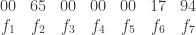
On the other hand, Richard Hamming is known for the Hamming codes, also frequently taught in a linear algebra course. This will be describes in more detail in one of the sections below, be here is the basic idea. In this scheme, developed in the 1940’s, we take a matrix G over a finite field F, constructed in a very particular way, and encode a message m by  , where the arithmetical operations are performed in F. The matrix G is called the generator matrix and c is the codeword transmitted to the receiver.
Here, in a nutshell, is the mystery at the heart of this post.
These schemes of Hill and Hamming, while algebraically very similar, have quite different aims. One is intended for secure communication, the other for reliable communication. However, in an unpublished paper [H5], Hill developed a hybrid encryption/error-detection scheme, what we shall call “Hill codes” (described in more detail below).
Why wasn’t Hill’s result published and therefore Hill, more than Hamming, known as a pioneer of error-correcting codes?
Perhaps Hill himself hinted at the answer. In an overly optimistic statement, Hill wrote (italics mine):
Further problems connected with checking operations in finite fields will be treated in another paper. Machines may be devised to render almost quite automatic the evaluation of checking elements  according to any proposed reference matrix of the general type described in Section 7, whatever the finite field in which the operations are effected. Such machines would enable us to dispense entirely with tables of any sort, and checks could be determined with great speed. But before checking machines could be seriously planned, the following problem — which is one, incidentally, of considerable interest from the standpoint of pure number theory — would require solution.
– Lester Hill, [H5]
By my interpretation, this suggests Hill wanted to answer the question below before moving on. As simple looking as it is, this problem is still, as far as I know, unsolved at the time of this writing.
Question 1 (Hill’s Problem):
Given k and q, find the largest r such that there exists a  van der Monde matrix with the property that every square submatrix is non-singular.
Indeed, this is closely related to the following related question from MacWilliams-Sloane [MS77], also still unsolved at this time. (Since Cauchy matrices do give a large family of matrices with the desired property, I’m guessing Hill was not aware of them.)
Question 2: Research Problem (11.1d)
Given k and q, find the largest r such that there exists a matrix having entries in GF(q) with the property that every square submatrix is non-singular.
In this post, after brief biographies, an even more brief description of the Hill cipher and Hamming codes is given, with examples. Finally, we reference previous blog posts where the above-mentioned unpublished paper, in which Hill discovered error-correcting codes, is discussed in more detail.
Short biographies
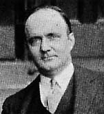
Who is Hill? Recent short biographies have been published by C. Christensen and his co-authors. Modified slightly from [C14] and [CJT12] is the following information.
Lester Sanders Hill was born on January 19, 1890 in New York. He graduated from Columbia University in 1911 with a B. A. in Mathematics and earned his Master’s Degree in 1913. He taught mathematics for a few years at Montana University, then at Princeton University. He served in the United States Navy Reserves during World War I. After the WWI, he taught at the University of Maine and then at Yale, from which he earned his Ph.D. in mathematics in 1926. His Ph.D. advisor is not definitely known at this writing but I think a reasonable guess is Wallace Alvin Wilson.
In 1927, he accepted a position with the faculty of Hunter College in New York City, and he remained there, with one exception, until his resignation in 1960 due to illness. The one exception was for teaching at the G.I. University in Biarritz in 1946, during which time he may have been reactivated as a Naval Reserves officer. Hill died January 9, 1961.
Thanks to an interview that David Kahn had with Hill’s widow reported in [C14], we know that Hill loved to read detective stories, to tell jokes and, while not shy, enjoyed small gatherings as opposed to large parties.
Who is Hamming? His life is much better known and details can be readily found in several sources.
Richard Wesley Hamming was born on February 11, 1915, in Chicago. Hamming earned a B.S. in mathematics from the University of Chicago in 1937, a masters from the University of Nebraska in 1939, and a PhD in mathematics (with a thesis on differential equations)
from the University of Illinois at Urbana-Champaign in 1942. In April 1945 he joined the Manhattan Project at the Los Alamos Laboratory, then left to join the Bell Telephone Laboratories in 1946. In 1976, he retired from Bell Labs and moved to the Naval Postgraduate School in Monterey, California, where he worked as an Adjunct Professor
and senior lecturer in computer science until his death on January 7, 1998.
Hill’s cipher
The Hill cipher is a polygraphic cipher invented by Lester S. Hill in 1920’s. Hill and his colleague Wisner from Hunter College filed a patent for a telegraphic device encryption and error-detection device which was roughly based on ideas arising from the Hill cipher. It appears nothing concrete became of their efforts to market the device to the military, banks or the telegraph company (see Christensen, Joyner and Torres [CJT12] for more details). Incidently, Standage’s excellent book [St98] tells the amusing story of the telegraph company’s failed attempt to add a relatively simplistic error-detection to telegraph codes during that time period.
Some books state that the Hill cipher never saw any practical use in the real world. However, research by historians F. L. Bauer and David Kahn uncovered the fact that the Hill cipher saw some use during World War II encrypting three-letter groups of radio call signs [C14]. Perhaps insignificant, at least compared to the practical value of Hamming codes, none-the-less, it was a real-world use.
The following discussion assumes an elementary knowledge of matrices. First, each letter is first encoded as a number, namely
 . The subset of the integers
  will be denoted by Z/26Z. This is closed under addition and multiplication (mod 26), and sums and products (mod 26) satisfy the usual associative and distributive properties. For R = Z/26Z, let GL(k,R) denote the set of invertible matrix transformations
  (that is, one-to-one and onto linear functions).
The construction
Suppose your message m consists of n capital letters, with no spaces. This may be regarded an n-tuple M with elements in R = Z/26Z. Identify the message M as a sequence of column vectors  . A key in the Hill cipher is a matrix K, all of whose entries are in R, such that the matrix K is invertible. It is important to keep K and k secret.
The encryption is performed by computing  and rewriting the resulting vector as a string over the same alphabet. Decryption is performed similarly by computing
  .
.
Example 1: Suppose m is the message “BWGN”. Transcoding into numbers, the plaintext is rewritten  . Suppose the key is
Using Hill’s encryption above gives  . (Verification is left to the reader as an exercise.)
Security concerns: For example, this cipher is linear and can be broken by a known plaintext attack.
Hamming codes
Richard Hamming is a pioneer of coding theory, introducing the binary
Hamming codes in the late 1940’s. In the days when an computer error could crash the computer and force the programmer to retype his punch cards, Hamming, out of frustration, designed a system whereby the computer could automatically correct certain errors. The family of codes named after him can easily correct one error.
Hill’s unpublished paper
While he was a student at Yale, Hill published three papers in Telegraph and Telephone Age [H1], [H2], [H3]. In these papers Hill described a mathematical method for checking the accuracy of telegraph communications. There is some overlap with these papers and [H5], so it seems likely to me that Hill’s unpublished paper [H5] dates from this time (that is, during his later years at Yale or early years at Hunter).
In [H5], Hill describes a family of linear block codes over a finite field and an algorithm for error-detection (which can be easily extended to error-correction). In it, he states the construction of what I’ll call the “Hill codes,” (defined below), gives numerous computational examples, and concludes by recording Hill’s Problem (stated above as Question 1). It is quite possibly Hill’s best work.
Here is how Hill describes his set-up.
Our problem is to provide convenient and practical accuracy checks upon
a sequence of n elements  in a finite algebraic
field F. We send, in place of the simple sequence , the amplified sequence 
consisting of the “operand” sequence and the “checking” sequence.
– Lester Hill, [H5]
Then Hill continues as follows. Let F=GF(p) denote the finite field having p elements, where  is a prime number. The checking sequence contains k elements of F as follows:

for  . The checks are to be determined by means of a
fixed matrix
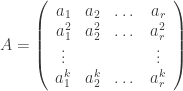
of elements of F, the matrix having been constructed according to the criteria in Hill’s Problem above. In other words, if the operand sequence (i.e., the message) is the vector  , then the amplified sequence (or codeword in the Hill code) to be transmitted is

where  and where
  denotes the
 identity matrix. The Hill code is the row space of G.
We conclude with one more open question.
Question 3:
What is the minimum distance of a Hill code?
The minimum distance of any Hamming code is 3.
Do all sufficiently long Hill codes have minimum distance greater than 3?
Summary
Most books today (for example, the excellent MAA publication written by Thompson [T83]) date the origins of the theory of error-correcting codes to the late 1940s, due to Richard Hamming. However, this paper argues that the actual birth is in the 1920s due to Lester Hill. Topics discussed include why Hill’s discoveries weren’t publicly known until relatively recently, what Hill actually did that trumps Hamming, and some open (mathematical) questions connected with Hill’s work.
For more details, see these previous blog posts.
Acknowledgements: Many thanks to Chris Christensen and Alexander Barg for
helpful and encouraging conversations. I’d like to explicitly credit Chris Christensen, as well as historian David Kahn, for the original discoveries of the source material.
Bibliography
[C14] C. Christensen, Lester Hill revisited, Cryptologia 38(2014)293-332.
[CJT12] ——, D. Joyner and J. Torres, Lester Hill’s error-detecting codes, Cryptologia 36(2012)88-103.
[H1] L. Hill, A novel checking method for telegraphic sequences, Telegraph and
Telephone Age (October 1, 1926), 456 – 460.
[H2] ——, The role of prime numbers in the checking of telegraphic communications, I, Telegraph and Telephone Age (April 1, 1927), 151 – 154.
[H3] ——, The role of prime numbers in the checking of telegraphic
communications, II, Telegraph and Telephone Age (July, 16, 1927), 323 – 324.
[H4] ——, Lester S. Hill to Lloyd B. Wilson, November 21, 1925. Letter.
[H5] ——, Checking the accuracy of transmittal of telegraphic communications by means of operations in finite algebraic fields, undated and unpublished notes, 40 pages.
(hill-error-checking-notes-unpublished)
[MS77] F. MacWilliams and N. Sloane, The Theory of Error-Correcting Codes, North-Holland, 1977.
[Sh] A. Shokrollahi, On cyclic MDS codes, in Coding Theory and Cryptography: From Enigma and Geheimschreiber to Quantum Theory, (ed. D. Joyner), Springer-Verlag, 2000.
[St98] T. Standage, The Victorian Internet, Walker & Company, 1998.
[T83] T. Thompson, From Error-Correcting Codes Through Sphere Packings to Simple Groups, Mathematical Association of America, 1983.
 according to any proposed reference matrix of the general type described in Section 7, whatever the finite field in which the operations are effected. Such machines would enable us to dispense entirely with tables of any sort, and checks could be determined with great speed. But before checking machines could be seriously planned, the following problem — which is one, incidentally, of considerable interest from the standpoint of pure number theory — would require solution:
 with
with  elements, and for the checking therein of
  -element sequence
  , a reference matrix
 is the greatest possible. Corresponding to any
 being elements of any given finite algebraic field
  with
with  — determinants of first order (
 ) being single elements of the matrix.
 ,
,  is an
is an  element operand
 -element check based upon the matrix
  is:
is:
 ,
,  .
. ,
,  be a
be a  , \dots, $f_{s}$, $s\leq n$. Let
  be a positive integer less than or equal to
  . If, in the transmittal of the sequence
 -in-
-in- chance of escaping disclosure, according as $v$ is, or is not, less than
  . In this statement,
  . The presence of error is evidently certain to be disclosed.
 . There is no loss of generality of we assume [This assumption implies
  . – wdj] the $v$ errors are
  ,
,  , affecting
  . The errors cannot escape disclosure. For, to do so, they would have to satisfy the system of homogeneous linear equations:
 contains no vanishing determinant of any order, and which, therefore admits no solution other than
  (
( ).
). errors fall among the
  and
and  errors fall among the
  . Without loss in generality, we may assume that the errors are
  , affecting
  , and
, and  ,
,  , affecting
  ,
,  .
. . Writing
  , where
  denotes a non-negative integer which may or may not be zero, we have
  . Hence
  of the
 denote a set of
  . But the matrix of coefficients in this system contains no vanishing determinant, so that the only solution would be
  ).
). . Then
  , where $h$ denotes a positive integer. Assuming that the presence of error is to escape detection, we see, therefore, that the
  ) a system of
  equations involving only the errors
  , (
, ( ) a system of
  equations involving all
  — as polynomial functions of the
  errors are determined as rational functions of the remaining
  errors determine the other $t$ errors.
 of elements of any given finite algebraic field. Operations in the field
  . Suppose that we wish, in a certain message, to transmit the numerical sequence

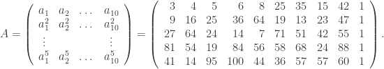
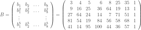
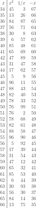
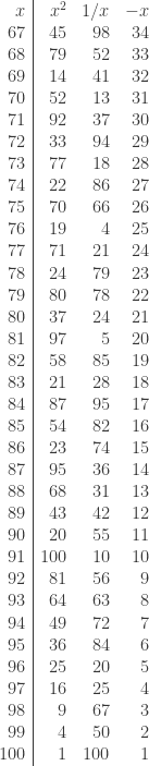
 ) is obtained by the simple tabulation which follows. We use Table 4, noting that in each of the nine rows, the one-hundred columns are shown in four sections, there being twenty-five columns in each section.


 , and a one-column tabulation would have sufficed. If a two-element check had been desired, we should have taken
  and a two-column tabulation would have sufficed. Etc.
 elements, the procedure, to determine check of Type A, is obvious. A
  , with
  , is as stated:
 . The manner of its evaluation, by means of Table 4, is clear.
 .
. – that is, upon
 . The tabulation is as follows:
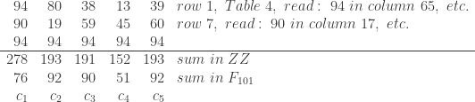
 . The tabulation is as follows:
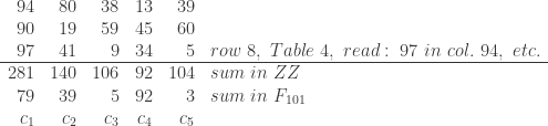


 , on the sequence
  of
of  , is given by
 , will be called a check of “type

 th row shows the products of all non-zero elements of
  ($i=1,2,\dots, 9$), where the
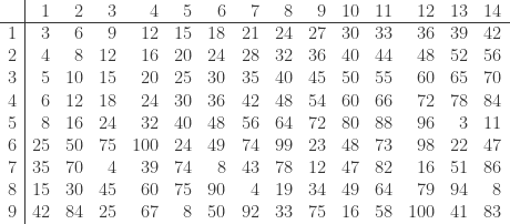
 be a polynomial
 denote the reciprocal polynomial
 . For example,


 do the polynomial roots
  lie on the unit circle
  ?
?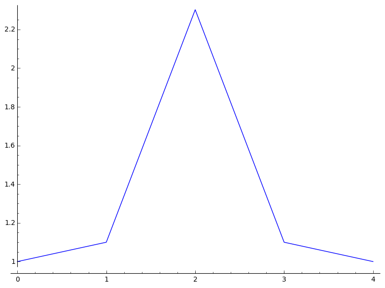
 and
and  and
and  the largest
  which has this roots property is as in the plot.
 the largest
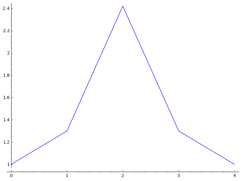
 the largest
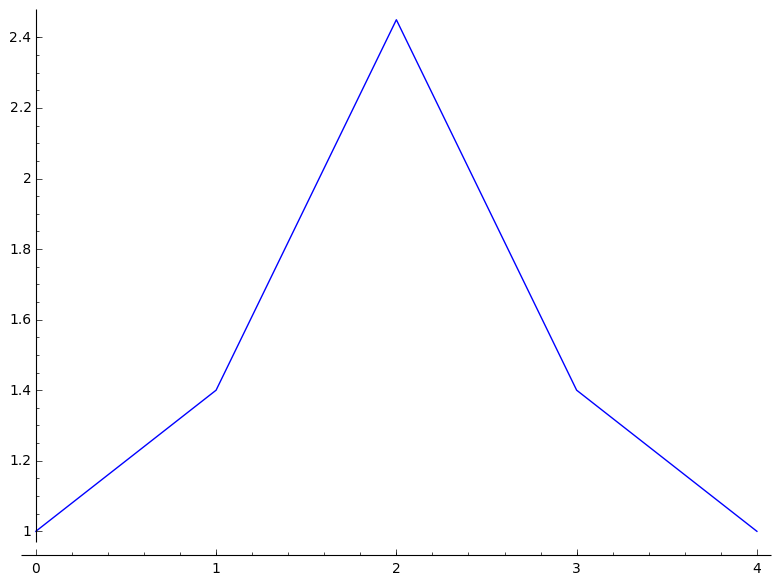
 the largest
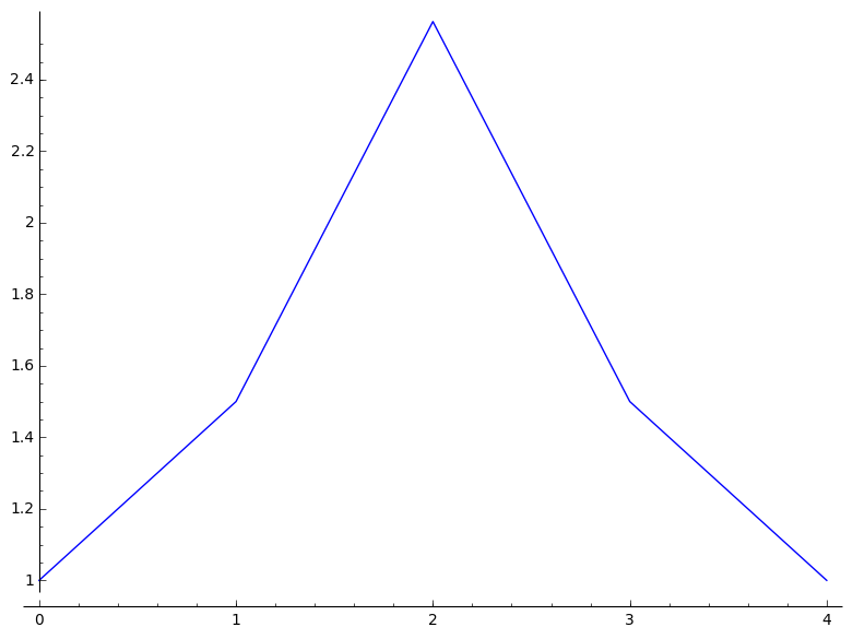
 the largest
  be a ”slowly increasing” function.
 , where
  , then the roots of
  all lie on the unit circle.
 , is symmetric increasing if and only if it can be written as a product of quadratics of the form
  , where all but one of the factors satisfy
  . One of the factors can be of the form
  , for some
  .
. in place of
  .}
.}  ,
,  ,
,  ,
, 


 . Determining the fractions in this manner, we write the two equations in the form:
 and
and 
 is very convenient to work with. The residue, modulo

 , and if at least one of the particular elements
  is correctly transmitted, the presence of error will certainly be disclosed. But if exactly three errors are made, affecting presicely the elements
  (
( ) chance of escaping disclosure.
 (
( ) chance of escaping disclosure.


 can be written
  , or
, or  .
.
 can be made quite arbitrarily. But then the values of
  and
and  are then completely determined. There is evidently a

 .
. is the only vanishing determinant of any order in the matrix employed, all other assertions made in (1′) and (2′) are readily justified. This will be made clear in the following sections.

 an arbitrary element of this field, we see that negatives and reciprocals of the elements of the field are as shown in the scheme:


 . By the usual methods, it is quickly found that one solution is (
 ,
,  ,
,  ). The general solution is (
 ,
,  ,
,  denotes an element of the field.
 ,
,  .
.
 . It may be observed in passing that if
 .
. ,
,  be
be  is given by the formula
 is the smallest non-negative integer satisfying


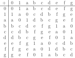
 elements. An addition table is not needed. The multiplication table is as follows:
 are negatives —
  ,
,  — when
  . In the present example, therefore, two marks
  are negatives if
 are momentarily regarded as ordinary integers of familiar arithmetic.
 . We shall use it in illustrating our checking operations.
 , so that we may write


 being irreducible in

 is not the square of an element in
You must be logged in to post a comment.