I recently learned about a new class of seemingly complicated, but in fact very simple functions which are called by several names, but perhaps most commonly as NCF Boolean functions (NCF is an abbreviation for “nested canalyzing function,” a term used by mathematical biologists). These functions were independently introduced by theoretical computer scientists in the 1960s using the term unate cascade functions. As described in [JRL2007] and [LAMAL2013], these functions have applications in a variety of scientific fields. This post describes these functions.
A Boolean function of n variables is simply a function . Denote the -vector space of such functions by . We write an element of this space as , where the variables will be called coordinate variables. Let
denote the restriction map sending to . In this post, the cosets
will be called coordinate hyperplanes (). A function in which is constant along some coordinate hyperplane is called canalyzing. An NCF function is a function which (a) is constant along some coordinate hyperplane , (b) whose restriction is constant along some coordinate hyperplane , (c) whose restriction is constant along some coordinate hyperplane , (d) and so on. This “nested” inductive definition might seem complicated, but to a computer it’s pretty simple and, to boot, it requires little memory to store.
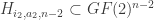
If and then let denote the vector whose i-th coordinate is flipped (bitwise). The sensitivity of at is . Roughly speaking, it’s the number of single-bit changes in that change the value of . The (maximum) sensitivity is the quantity The block sensitivity is defined similarly, but you allow blocks of indices of coordinates to by flipped bitwise, as opposed to only one. It’s possible to
compute the sensitivity of any NCF function,
show the block sensitivity is equal to the sensitivity,
compute the cardinality of the set of all monotone NCF functions.
For details, see for example Li and Adeyeye [LA2012].
This is a very short introductory survey of graph-theoretic properties of Boolean functions.
I don’t know who first studied Boolean functions for their own sake. However, the study of Boolean functions from the graph-theoretic perspective originated in Anna Bernasconi‘s thesis. More detailed presentation of the material can be found in various places. For example, Bernasconi’s thesis (e.g., see [BC]), the nice paper by P. Stanica (e.g., see [S], or his book with T. Cusick), or even my paper with Celerier, Melles and Phillips (e.g., see [CJMP], from which much of this material is literally copied).
For a given positive integer , we may identify a Boolean function
with its support
For each , let denote the set of complements , for , and let denote the complementary Boolean function. Note that
where denotes the complement of in . Let
denote the cardinality of the support. We call a Boolean function even (resp., odd) if is even (resp., odd). We may identify a vector in with its support, or, if it is more convenient, with the corresponding integer in Let
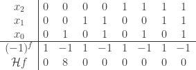
be the binary representation ordered with least significant bit last (so that, for example, ).
Let denote the $2^n\times 2^n$ Hadamard matrix defined by , for each such that . Inductively, these can be defined by
The Walsh-Hadamard transform of is defined to be the vector in whose th component is
where we define as the column vector where the th component is
for .
Example
A Boolean function of three variables cannot be bent. Let be defined by:
In her thesis, Bernasconi found a relationship between the spectrum of the Cayley graph ,
(the eigenvalues of the adjacency matrix ) to the Walsh-Hadamard transform . Note that and are related by the equation where . She discovered the relationship
between the spectrum of the Cayley graph of a Boolean function and the values of the Walsh-Hadamard transform of the function. Therefore, the spectrum of , is explicitly computable as an expression in terms of .
References:
[BC] A. Bernasconi and B. Codenotti, Spectral analysis of Boolean functions as a graph eigenvalue problem, IEEE Trans. Computers 48(1999)345-351.


 , we may identify a Boolean function

 , let
, let  denote the set of complements
  , for
, for  , and let
  denote the complementary Boolean function. Note that
 denotes the complement of
  in
in  . Let
. Let
 is even (resp., odd). We may identify a vector in
  Let
Let
 ).
). denote the $2^n\times 2^n$ Hadamard matrix defined by
 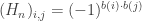 , for each
  such that
  . Inductively, these can be defined by
 is defined to be the vector in
  whose
whose  th component is
 as the column vector where the
  th component is
 .
.
 . It is even because
 be the Cayley graph of
 so
so  has no loops. In this case,
  -regular graph having
  connected components, where
 , the set of neighbors
  of
of  is given by
 be the
  adjacency matrix of


 of the adjacency matrix
  ) to the Walsh-Hadamard transform
  . Note that
  where
where  . She discovered the relationship

You must be logged in to post a comment.