A matroid M is specified by a set X of “points” and a collection B of “bases, where  , satisfying certain conditions (see, for example, Oxley’s book, Matroid theory).
One way to construct a matroid, as it turns out, is to consider a matrix M with coefficients in a field F. The column vectors of M are indexed by the numbers  . The collection B of subsets of J associated to the linearly independent column vectors of M of cardinality
 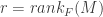 forms a set of bases of a matroid having points
  .
.
How do you compute B? The following Sage code should work.
def independent_sets(mat):
    """
    Finds all independent sets in a vector matroid.

    EXAMPLES:
        sage: M = matrix(GF(2), [[1,0,0,1,1,0],[0,1,0,1,0,1],[0,0,1,0,1,1]])
        sage: M
        [1 0 0 1 1 0]
        [0 1 0 1 0 1]
        [0 0 1 0 1 1]
        sage: independent_sets(M)
        [[0, 1, 2], [], [0], [1], [0, 1], [2], [0, 2], [1, 2],
        [0, 1, 4], [4], [0, 4], [1, 4], [0, 1, 5], [5], [0, 5],
        [1, 5], [0, 2, 3], [3], [0, 3], [2, 3], [0, 2, 5], [2, 5],
        [0, 3, 4], [3, 4], [0, 3, 5], [3, 5], [0, 4, 5], [4, 5],
        [1, 2, 3], [1, 3], [1, 2, 4], [2, 4], [1, 3, 4], [1, 3, 5],
        [1, 4, 5], [2, 3, 4], [2, 3, 5], [2, 4, 5]]
        sage: M = matrix(GF(3), [[1,0,0,1,1,0],[0,1,0,1,0,1],[0,0,1,0,1,1]])
        sage: independent_sets(M)
        [[0, 1, 2], [], [0], [1], [0, 1], [2], [0, 2], [1, 2],
        [0, 1, 4], [4], [0, 4], [1, 4], [0, 1, 5], [5], [0, 5],
        [1, 5], [0, 2, 3], [3], [0, 3], [2, 3], [0, 2, 5], [2, 5],
        [0, 3, 4], [3, 4], [0, 3, 5], [3, 5], [0, 4, 5], [4, 5],
        [1, 2, 3], [1, 3], [1, 2, 4], [2, 4], [1, 3, 4], [1, 3, 5],
        [1, 4, 5], [2, 3, 4], [2, 3, 5], [2, 4, 5], [3, 4, 5]]
        sage: M345 = matrix(GF(2), [[1,1,0],[1,0,1],[0,1,1]])
        sage: M345.rank()
        2
        sage: M345 = matrix(GF(3), [[1,1,0],[1,0,1],[0,1,1]])
        sage: M345.rank()
        3
    """
    F = mat.base_ring()
    n = len(mat.columns())
    k = len(mat.rows())
    J = Combinations(n,k)
    indE = []
    for x in J:
        M = matrix([mat.column(x[0]),mat.column(x[1]),mat.column(x[2])])
        if k == M.rank():     # all indep sets of max size
            indE.append(x)
            for y in powerset(x): # all smaller indep sets
                if not(y in indE):
                    indE.append(y)
    return indE

def bases(mat, invariant = False):
    """
    Find all bases in a vector/representable matroid.

    EXAMPLES:
        sage: M = matrix(GF(2), [[1,0,0,1,1,0],[0,1,0,1,0,1],[0,0,1,0,1,1]])
        sage: bases(M)

        [[0, 1, 2],
         [0, 1, 4],
         [0, 1, 5],
         [0, 2, 3],
         [0, 2, 5],
         [0, 3, 4],
         [0, 3, 5],
         [0, 4, 5],
         [1, 2, 3],
         [1, 2, 4],
         [1, 3, 4],
         [1, 3, 5],
         [1, 4, 5],
         [2, 3, 4],
         [2, 3, 5],
         [2, 4, 5]]
        sage: L = [x[1] for x in bases(M, invariant=True)]; L.sort(); L
         [5, 16, 17, 33, 37, 44, 45, 48, 81, 84, 92, 93, 96, 112, 113, 116]
    """
    r = mat.rank()
    ind = independent_sets(mat)
    B = []
    for x in ind:
        if len(x) == r:
            B.append(x)
    B.sort()
    if invariant == True:
        B = [(b,sum([k*2^(k-1) for k in b])) for b in B]
    return B


 , where V is the set of vertices and E a set of ordered pairs of distinct vertices representing the edges, and, for each edge an “orientation”. Simply put, an orientation on $\latex \Gamma$ is a list
  of length |E| consisting of
  ‘s. If an edge e=(v,w) is associated to a -1 then we think of the edge as going from w to v; otherwise, it goes from v to w.
 and let
  . The incidence matrix may be regarded as a mapping B from the vector space of function on V to the vector space of functions on E:
 ,
, with the vector space of column vectors
  and
and  with the vector space of column vectors
  then B may be regarded as an
  matrix.

 :
:
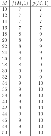
 for different values of
  (see R. Hill, J. Karim, E. Berlekamp, “The solution of a problem of Ulam on searching with lies,” IEEE, 1998):
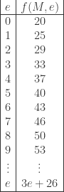


You must be logged in to post a comment.