Mathematical notes on Depth of Field

Posted on 2013/05/27 by wdjoyner

There are a million blog posts on photography depth of field (DOF). This one makes a million and one! If writing this will help me, and hopefully someone else, understand it better, it will be worth it.

We assume that a typical camera lens is fixed in space and represents the properties of a “thin convex lens in air”. We say an object, such as a distant mountain, is at infinity if light from it enters the lens along a ray perpendicular, or nearly perpendicular, to the lens plane. The principal focal point is that point behind the lens that an object at infinity (on the axis of the lens) focuses to. 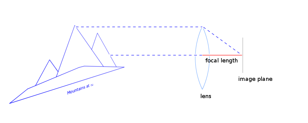The focal length $f$ is the distance from the center of the lens to the principal focal point of the lens. This is illustrated below.

mountains “at infinity” with respect to lens, created using GIMP and Sage

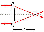
Focal length for a convex lens (source: Wikipedia)

Define the object plane to be the plane of the object you are photographing parallel to the plane of the lens) and want to look sharp in your photo. (Again, the object is assumed to be on the axis of the lens.) The light from the object converges behind the lens to a small region called the image. The image plane is a plane (parallel to the lens) which intersects this image region. You want the plane of the digital sensor (or camera film) to be at or very near the image plane, or else the photo will not have the object in focus.

We assume that the camera is a projective transformation from the plane of the object to the plane of the digital sensor. In other words, we assume that the camera has the property that if it focuses on a (stright) line or circle then it captures a line or circle on the film or digital sensor. (Of course, in reality, the lens imperfections and the light diffraction have an effect, but this hypothesis is nearly true in many cases.)

Consider an object at infinity (say, some distant mountains) in the plane of the plane of your lens. Suppose your camera’s digital sensor is located in the same plane as the image plane, so that the mountains will be in focus in your camera. The distance from the lens to the sensor plane is the focal length $f$ . Consider the light entering your lens from a small disk (also on the axis of the lens) at a distance $u$ in front of the lens. This light will meet the sensor plane but its image in the photo, depending on the value of $u$ , may or may not be in focus. If the disk is relatively small in diameter then its blurred image on the photo is sometimes called a circle of confusion. Concretely speaking, the circle of confusion measures the maximum diameter on an 8′′ × 10′′ photo for which there is an acceptable blur in the image of the disk. Suppose now that the distance between the lens and sensor plane (say that the lens, along with the disk in front of it, are fixed but the sensor plane is translated backwards) is increased until this small disk is in focus in the photo. Call this new distance between the lens and the sensor plane $v$ .

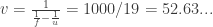
Lemma 1. The focal length $f$ , the distance from the lens to the object to photograph $u$ , and the distance from lens to the image focus plane $v$ are then related by the lens equation $\frac{1}{u}+\frac{1}{v}=\frac{1}{f}$ .

Example: As $v$ is decreased, $u$ must be increased. For example, consider a normal lens for a 35 mm camera with a focal length of $f = 50$ mm. To focus an object 1 m away ( $u = 1000$ mm), we solve for $v = \frac{1}{\frac{1}{f}-\frac{1}{u}} = 1000/19 = 52.63...$ . Therefore, the lens must be moved 2.6 mm further away from the image plane, to $v = 52.6$ mm.

The depth of field (DOF) is the portion of a scene that appears sharp in the image. More precisely, it is the area near the object plane in which the circles of confusion are acceptably small (where “acceptably small” has some precise pre-defined meaning, e.g., 0.2mm for a photo blown up to an 8′′ × 10′′ print). Although a lens can precisely focus at only one distance, the decrease in sharpness is gradual on either side of the focused distance, so that within the DOF, the unsharpness is imperceptible under normal viewing conditions. See the image below for an example of an image with a “small” (or “short”) DOF.

snowflake, small DOF example

The lens aperture is the circular opening in the lens allowing light to pass through. The actual diameter of opening is called the effective aperture. By convention, the aperture is measured as a quotient relative to the focal length $f$ . For example, the aperture $f/2$ is an opening which is half the focal length, so if $f = 50$ mm then the effective aperture would be a disc of diameter 25mm. In general, if the aperture is $f/N$ (read “the f-stop is N”, where $N \geq 1$ ) then $N$ is called the f-number or f-stop. Two apertures (or f-stops) are said to differ by a full stop if they differ by a factor of $\sqrt{2}$ . Usually the stop numbers fall into the sequence

$1, \sqrt{2}, 2, 2\sqrt{2}, 4, 4\sqrt{2}, 8, 8\sqrt{2}, 16, 16\sqrt{2}, 32, 32\sqrt{2}, ...,$

which might be rounded up or down to

$1, 1.4, 2, 2.8, 4, 5.6, 8, 11, 16, 22, 32, 45, ....$

The larger f-stop is, the smaller the aperture.

An aperture slide card for an old-fashioned camera.

For more details, see for example:

Jeff Conrad, Depth of field in depth, preprint 2006. Available at: http://www.largeformatphotography.info/.
L. Evens, View camera geometry, preprint, 2008.
R. E. Wheeler, Notes on view camera geometry, preprint, 2003.

Paley graphs in Sage

Posted on 2013/03/06 by wdjoyner

Let $q$ be a prime power such that $q\equiv 1 \pmod 4$ . Note that this implies that the unique finite field of order $q$ , $GF(q)$ , has a square root of $-1$ . Now let $V=GF(q)$ and

$E = \{(a,b)\in V\times V\ |\ a-b\in GF(q)^2\}.$
By hypothesis, $(a,b)\in E$ if and only if $(b,a)\in E$ . By definition $G = (V, E)$ is the Paley graph of order $q$ .

Paley was a brilliant mathematician who died tragically at the age of 26. Paley graphs are one of the many spin-offs of his work. The following facts are known about them.

The eigenvalues of Paley graphs are $\frac{q-1}{2}$ (with multiplicity $1$ ) and
$\frac{-1 \pm \sqrt{q}}{2}$ (both with multiplicity $\frac{q-1}{2}$ ).
It is known that a Paley graph is a Ramanujan graph.
It is known that the family of Paley graphs of prime order is a vertex expander graph family.
If $q=p^r$ , where $p$ is prime, then $Aut(G)$ has order $rq(q-1)/2$ .

Here is Sage code for the Paley graph (thanks to Chris Godsil, see [GB]):

def Paley(q):
    K = GF(q)
    return Graph([K, lambda i,j: i != j and (i-j).is_square()])

(Replace “K” by “ $K.\langle a\rangle$ ” above; I was having trouble rendering it in html.) Below is an example.

sage: X = Paley(13)
sage: X.vertices()
[0, 1, 2, 3, 4, 5, 6, 7, 8, 9, 10, 11, 12]
sage: X.is_vertex_transitive()
True
sage: X.degree_sequence()
[6, 6, 6, 6, 6, 6, 6, 6, 6, 6, 6, 6, 6]
sage: X.spectrum()
[6, 1.302775637731995?, 1.302775637731995?, 1.302775637731995?,
1.302775637731995?, 1.302775637731995?, 1.302775637731995?,
-2.302775637731995?, -2.302775637731995?, -2.302775637731995?,
-2.302775637731995?, -2.302775637731995?, -2.302775637731995?]
sage: G = X.automorphism_group()
sage: G.cardinality()
78

We see that this Paley graph is regular of degree $6$ , it has only three distinct eigenvalues, and its automorphism group is order $13\cdot 12/2 = 78$ .

Here is an animation of this Paley graph:

The frames in this animation were constructed one-at-a-time by deleting an edge and plotting the new graph.

Here is an animation of the Paley graph of order $17$ :

The frames in this animation were constructed using a Python script:

X = Paley(17)
E = X.edges()
N = len(E)
EC = X.eulerian_circuit()
for i in range(N):
    X.plot(layout="circular", graph_border=True, dpi=150).save(filename="paley-graph_"+str(int("1000")+int("%s"%i))+".png")
    X.delete_edge(EC[i])
X.plot(layout="circular", graph_border=True, dpi=150).save(filename="paley-graph_"+str(int("1000")+int("%s"%N))+".png")

Instead of removing the frames “by hand” they are removed according to their occurrence in a Eulerian circuit of the graph.

Here is an animation of the Paley graph of order $29$ :

[GB] Chris Godsil and Rob Beezer, Explorations in Algebraic Graph Theory with Sage, 2012, in preparation.

Mathematics Problem, #120

Posted on 2013/03/06 by wdjoyner

A colleague Bill Wardlaw (March 3, 1936-January 2, 2013) used to create a “Problem of the Week” for his students, giving a prize of a cookie if they could solve it. Here is one of them.

Mathematics Problem, #120

A calculus 1 student Joe asks another student Bob “Is the following expression correct?” and writes

$f'(x^3)=3x^2$
on the blackboard. Bob replies, “Well, it could be, but I don’t think that is what you mean.”

Find a function that makes what Joe said correct.

Solution to #119:
There are $(16!)/(2^8)$ (about 82 billion) different orders that the spider can put on shoes and socks.

Lester Hill’s “The checking of the accuracy …”, part 8

Posted on 2013/03/03 by wdjoyner

Introductory example of checking

We may use the field $F_{23}$ as the basis for a simple illustrative exercise in the actual procedure of checking. The general of the operations involved will thus be made clear, so far as modus operandi is concerned, and we shall be enabled to discuss more easily the pertinent mathematical details.

It is easy to set up telegraphic codes of high capacity using combinations of four letters each which are not required to be pronounceable. In fact, a sufficiently high capacity may be obtained when only
twenty-three letters of the alphabet are used at all. Hence we can omit any three letters whose Morse equivalents (dot-dash) are most frequently used. Let us suppose that we have before us a code of this kind which employs the letters

$A\ \ B\ \ C\ \ E\ \ F\ \ G\ \ H\ \ I\ \ J\ \ L\ \ M\ \ N\ \ P\ \ Q\ \ R\ \ S\ \ T\ \ U\ \ V\ \ W\ \ X\ \ Y\ \ Z$
and avoids, for reasons stated of for some good reason, the three letters

$D\ \ K\ \ O\, .$

Suppose that, by prearrangement with telegraphic correspondents, the letters used are paired in
an arbitrary, but fixed, way with the thwenty-three elements of $F_{23}$ .
Let the pairings be, for instance:

$\begin{tabular}{ccccccccccccccccccccccc} A & B & C & E & F & G & H & I & J & L & M & N & P & Q & R & S & T & U & V & W & X & Y & Z \\ \hline 4 & 7 & 9 & 14& 2 & 1 & 11 & 15 & 10 & 3 & 19 & 18 & 21 & 16 & 6 & 20 & 17 & 12 & 0 & 22 & 5 & 13 & 8 \\ \end{tabular}$
or, in numerical arrangement:

$\begin{tabular}{ccccccccccccccccccccccc} 0 & 1 & 2 & 3 & 4 & 5 & 6 & 7 & 8 & 9 & 10 & 11 & 12 & 13 & 14 & 15 & 16 & 17 & 18 & 19 & 20 & 21 & 22 \\ \hline V & G & F & L& A & X & R & B & Z & C & J & H & U & Y & E & I & Q & T & N & M & S & P & W \\ \end{tabular}$

A four-letter group (code word), such as EZRA or XTYP, will indicate a definite entry of a specific page of a definite code volume, several such volumes being perhaps employed in the code. An entry will, in general, be a phrase of sentence, or a group of phrases or sentences, commonly occurring in the class of messages for which the code has been constructed.

Suppose that we have agreed to provide, in our messages, three-letter checks upon groups of twelve letters; in other words, to check in one operation a sequence of three four-letter code words. The twelve letters of the three code words are thus expanded to fifteen; but we send just three telegraphic words — three combinations of five letters, each of which is, in general, unpronounceable.

For illustration, let the first three code words of a message be:

$XTYP\ \ \ \ VZRV\ \ \ \ HVHH$
The corresponding sequence of paired elements in $F_{23}$ is:

$5 \ \ 17\ \ 13\ \ 21\ \ 0\ \ 8\ \ 6\ \ 0\ \ 11\ \ 0\ \ 11\ \ 11.$
This is our operand sequence $f_i$ :

$f_1 = 5,\ \ f_2=17,\ \ f_3=13,\ \ f_4=21,\ \ f_5=0,\ \dots,\ ,f_{12}=11.$

Let us determine the checking matrix $c_1, c_2, c_3$ by using as reference matrix

$\left( \begin{array}{cccccccccccc} 1 & 2 & 3 & 4 & 5 & 6 & 7 & 8 & 9 & 10 & 11 & 12\\ 1^2 & 2^2 & 3^2 & 4^2 & 5^2 & 6^2 & 7^2 & 8^2 & 9^2 & 10^2 & 11^2 & 12^2 \\ 1^3 & 2^3 & 3^3 & 4^3 & 5^3 & 6^3 & 7^3 & 8^3 & 9^3 & 10^3 & 11^3 & 12^3 \\ \end{array} \right)$
Thus the $c_j$ are to be

$c_j = \sum_{i=1}^{12} i^jf_i\ \ \ \ (j = 1,2,3),$

$c_1 = \sum_{i=1}^{12} if_i.\ \ \ c_2 = \sum_{i=1}^{12} i^2f_i.\ \ \ c_3 = \sum_{i=1}^{12} i^3f_i.$

Referring to the multiplication table of $F_{23}$ , we easily compute the $c_j$ .

For the first element $5$ , of the operant sequence $f_i$ , write

$\begin{tabular}{ccc} 5 & 5 & 5\\ \end{tabular}$

For the second element $17$ place a sheet of paper (or a ruler) under the second row
of the multiplication table, and in that row read: $11$ in column $17$ , $22$ in column $11$ , $21$ in column $22$ . we now have a second line for the tabular scheme:

$\begin{tabular}{ccc} 5 & 5 & 5\\ 11 & 22 & 21 \\ \end{tabular}$

For the third element $13$ place a sheet of paper (or a ruler) under the third row
of the multiplication table, and in that row read: $16$ in column $13$ , $2$ in column $16$ , $6$ in column $2$ . We now have the scheme:

$\begin{tabular}{ccc} 5 & 5 & 5\\ 11 & 22 & 21 \\ 16 & 2 & 6 \\ \end{tabular}$

The fifth, eighth, and tenth rows of the table will not be used, since
$f_5=f_8=f_{10}=0$ . The complete scheme is readily found to be:

$\begin{tabular}{cccc} 5 & 5 & 5 & \\ 11 & 22 & 21 & \\ 16 & 2 & 6 & \\ 15 & 14 & 10 & \\ 2 & 12 & 3 & \\ 19 & 18 & 11 & \\ 7 & 17 & 15 & \\ 6 & 20 & 13 & \\ 17 & 20 & 10 & \\ \hline 98 & 130 & 94 & sum in ZZ\\ 6 & 15 & 2 & sum in F-23\\ \end{tabular}$

We have $c_1=6$ , $c_2=15$ , $c_2=2$ .

We transmit, of course, the sequence of letters paired, in our system of communications, with the elements of the sequence,

$f_1\ f_2\ \dots f_{12}\ c_1\ c_2 \ c_3.$

Thus we transmit the sequence of letters: XTYP VZRV HVHH RIF; but we may conveniently agree to transmit it in the arrangement:

$XTYPR\ \ \ VZRVI\ \ \ HVHHF ,$

or in some other arrangement which employs only three telegraphic words (unpronounceable five letter groups).

We could have used other reference matrices, but we shall not stop to discuss this point. We may remark, however, that if the matrix

$\left( \begin{array}{cccccccccccc} 1 & 1 & 1 & 1 & 1 & 1 & 1 & 1 & 1 & 1 & 1 & 1 \\ 1 & 2 & 3 & 4 & 5 & 6 & 7 & 8 & 9 & 10 & 11 & 12\\ 1^2 & 2^2 & 3^2 & 4^2 & 5^2 & 6^2 & 7^2 & 8^2 & 9^2 & 10^2 & 11^2 & 12^2 \\ \end{array} \right)$

had been adopted, the checking elements would have been

$c_1 = \sum_{i=1}^{12} f_i.\ \ \ c_2 = \sum_{i=1}^{12} if_i.\ \ \ c_3 = \sum_{i=1}^{12} i^2f_i;$

and their evaluation would have been accomplished with equal
ease by means of the multiplication table of $F_{23}$ .

Problem of the Week, #119

Posted on 2013/02/09 by wdjoyner

A colleague Bill Wardlaw (March 3, 1936-January 2, 2013) used to create a “Problem of the Week” for his students, giving a prize of a cookie if they could solve it. Here is one of them.

PROBLEM 119

A spider puts on $8$ identical socks and $8$ identical shoes (and of course the spider has $8$ feet). In how many different ways can the spider do this, given that on each foot, the sock has to go on before the shoe?

Problem of the Week, #118

Posted on 2013/02/03 by wdjoyner

A colleague Bill Wardlaw (March 3, 1936-January 2, 2013) used to create a “Problem of the Week” for his students, giving a prize of a cookie if they could solve it. Here is one of them.

PROBLEM 118

Suppose that you draw numbers $x_1,x_2,\dots$ from $[0,1]$ randomly until $x_1+x_2+\dots +x_n$ first exceeds $1$ . What is the probability that this happens on the fourth draw? That is, what is the probability that $x_1+x_2+x_3 < 1$ and $x_1+x_2+x_3+x_4 > 1$ ?

PROBLEM 118A

In the above problem, what is the expected number of draws until the sum first exceeds $1$ ?

Problem of the Week, #117

Posted on 2013/01/28 by wdjoyner

A colleague Bill Wardlaw (March 3, 1936-January 2, 2013) used to create a “Problem of the Week” for his students, giving a prize of a cookie if they could solve it. Here is one of them.

PROBLEM 117

What is the largest number of regions $r(n)$ that a plane is divided into by $n$ straight lines in the plane?
Give $r(n)$ as a function of $n$ and explain why your answer is correct.

PROBLEM 117A

What is the largest number of regions $r(n, d)$ that $d$ -dimensional Euclidean space is divided into by $n$ hyperplanes?
Give $r(n, d)$ as a function of $n$ and $d$ , and find formulas for $b(n, d)$ , the number of regions that are bounded, and for $u(n, d)$ , the number of regions that are unbounded.
Of course, $r(n, d) = b(n, d) + u(n, d).$ Explain why these numbers are correct.

Problem of the Week, #116

Posted on 2013/01/24 by wdjoyner

A colleague Bill Wardlaw (March 3, 1936-January 2, 2013) used to create a “Problem of the Week” for his students, giving a prize of a cookie if they could solve it. Here is one of them.

PROBLEM 116

Bob invites Joe to see his new program, which prints $2 \times 2$ matrices with random integer entries. (These entries are as likely to be even as to be odd.) Joe, being a bit of a gambler, wants to bet Bob a dollar that the next matrix will have an even determinant. Should Bob take the bet? What is the probability that the next matrix will have an even determinant?

Note:
The determinant of the 2 x 2 matrix

$A = \left( \begin{array}{cc} a & b \\ c & d \\ \end{array} \right)$

is given by $det(A) = ad - bc$ .

ADVANCED PROBLEM 116A

What is the probability that the determinant of an $n \times n$ matrix with randomly chosen integer entries is divisible by the prime number $p$ ?
(Assume that the residues $0, 1, 2, ... , p-1$ are equally likely for each integer entry.)

The strange story of ternary bent functions in 2 variables

Posted on 2012/12/29 by wdjoyner

Consider a function $f:GF(3)^2\to GF(3)$ .

Such functions are often studied in terms of their Walsh(-Hadamard) transforms – a complex-valued function on $V=GF(3)^2$ that can be defined as

$W_f(u) = \sum_{x \in V} \zeta^{f(x)- \langle u,x\rangle},$
where $\zeta = e^{2\pi i/3}$ . We call $f$ bent if
$|W_f(u)|=3^{n/2},$
for all $u\in V$ (here $n=2$ ). Such ternary (or $3$ -ary) bent functions have been studied by a number of authors. Here we shall only consider those ternary bent functions of two variables which are even (in the sense $f(-x)=f(x)$ ) and $f(\vec{0})=0$ .

Thanks to a Sage computation, there are precisely $18$ such functions.

$\begin{array}{cccccccccc} {\rm bents}\backslash GF(3)^2 & (0, 0) & (1, 0) & (2, 0) & (0, 1) & (1, 1) & (2, 1) & (0, 2) & (1, 2) & (2, 2) \\ \hline b1 & 0 & 1 & 1 & 1 & 2 & 2 & 1 & 2 & 2 \\ b2 & 0 & 2 & 2 & 1 & 0 & 0 & 1 & 0 & 0 \\ b3 & 0 & 1 & 1 & 2 & 0 & 0 & 2 & 0 & 0 \\ b4 & 0 & 2 & 2 & 0 & 1 & 0 & 0 & 0 & 1 \\ b5 & 0 & 0 & 0 & 2 & 1 & 0 & 2 & 0 & 1 \\ b6 & 0 & 1 & 1 & 0 & 2 & 0 & 0 & 0 & 2 \\ b7 & 0 & 0 & 0 & 1 & 2 & 0 & 1 & 0 & 2 \\ b8 & 0 & 2 & 2 & 0 & 0 & 1 & 0 & 1 & 0 \\ b9 & 0 & 0 & 0 & 2 & 0 & 1 & 2 & 1 & 0 \\ b10 & 0 & 2 & 2 & 2 & 1 & 1 & 2 & 1 & 1 \\ b11 & 0 & 0 & 0 & 0 & 2 & 1 & 0 & 1 & 2 \\ b12 & 0 & 2 & 2 & 1 & 2 & 1 & 1 & 1 & 2 \\ b13 & 0 & 1 & 1 & 2 & 2 & 1 & 2 & 1 & 2 \\ b14 & 0 & 1 & 1 & 0 & 0 & 2 & 0 & 2 & 0 \\ b15 & 0 & 0 & 0 & 1 & 0 & 2 & 1 & 2 & 0 \\ b16 & 0 & 0 & 0 & 0 & 1 & 2 & 0 & 2 & 1 \\ b17 & 0 & 0 & 0 & 0 & 0 & 0 & 0 & 0 & 0 \\ b18 & 0 & 1 & 1 & 2 & 1 & 2 & 2 & 2 & 1 \\ \end{array}$

The (edge-weighted) Cayley graph of the second function $b_2$ is shown here (thanks to Sage):

cayley graph GF3 bent

When I showed this (actually, not just this graph but the print-outs of most of these Cayley graphs) to my colleague T.S. Michael, he observed that there is only one (up to iso) strongly regular (unweighted) graph of degree $4$ with $9$ vertices, and this is it!

Here are some relationships they satisfy:

$b_1=-b_{10}, \ \ b_2=-b_3, \ \ b_4 = -b_6, \ \ b_5 = -b_7, \ \ b_8=-b_{14},$

$b_9=-b_{15}, \ \ b_{11}=-b_{16}, \ \ b_{12}=-b_{18}, \ \ b_{13}=-b_{17},$

$b_1 = b_7+b_{14} = b_6+b_{15}, \ \ b_{10} = b_{4}+b_{9} = b_{5}+b_{8}, \ \ b_{12} = b_{2}+b_{11} = b_{7}+b_{8},$

$b_{13} = b_{3}+b_{11} = b_{6}+b_{9}, \ \ b_{17} = b_{2}+b_{16} = b_{4}+b_{15,}\ \ b_{18} = b_{3}+b_{16} = b_{5}+b_{14}.$

Their supports are given as follows:

$\{1,2,3,6\} = supp(b_2)=supp(b_3), \ \ \{1,2,4,8\} = supp(b_4)=supp(b_6),$

$\{1,2,5,7\} = supp(b_8)=supp(b_{14}), \ \ \{3,5,6,7\} = supp(b_9)=supp(b_{15}),$

$\{3,4,6,8\} = supp(b_{5})=supp(b_{7}),\ \ \{4,5,7,8\} = supp(b_{11})=supp(b_{16}),$

$\{1,2,3,4,5,6,7,8\} = supp(b_{1})=supp(b_{10}) = supp(b_{12})=supp(b_{13}) = supp(b_{17})=supp(b_{18}).$

Note that all these functions are weight $4$ or weight $8$ .

In fact, my colleague David Phillips and I found that if you consider their set of supports (together with the emptyset $\emptyset$ ),

$S = \{ \emptyset \} \cup \{ {\rm supp}(f)\ |\ f:GF(3)^2\to GF(3), \ f(0)=0,\ f\ {\rm bent} \},$
then $S$ forms a group under the symmetric difference operator $\Delta$ ! In fact, $S\cong GF(2)^3$ .

I told you this was strange!

The Sage code for this is rather involved but it can be found here: hadamard_transform.sage.

[1] Sage, mathematics software, sagemath.com.

A particularly simple puzzles on round pegs

Posted on 2012/12/24 by wdjoyner

I just thought of this simple (at least I think it is simple) puzzle.

Consider a long loop of string and a number (at least 2) of round pegs of radius 1 inch each, parallel to each other. Drape the string around the pegs and pull the pegs so that the string is tight, as in the picture (which has only 3 pegs). Notice some sections of the string are straight and some are curved (shown in red in the picture).

Why is the total length of the curved sections equal to $2\pi$ ?

This is related to a pulley puzzle of Harry Langman, published in 1949.

Yet Another Mathblog

Category Archives: math

Mathematical notes on Depth of Field

Paley graphs in Sage

Mathematics Problem, #120

Lester Hill’s “The checking of the accuracy …”, part 8

Problem of the Week, #119

PROBLEM 119

Problem of the Week, #118

PROBLEM 118

PROBLEM 118A

Problem of the Week, #117

PROBLEM 117

PROBLEM 117A

Problem of the Week, #116

PROBLEM 116

ADVANCED PROBLEM 116A

The strange story of ternary bent functions in 2 variables

A particularly simple puzzles on round pegs