Mathematical romantic?

Posted on 2008/07/26 by wdjoyner

A colleague Bill Wardlaw (Robert Steinberg’s 2nd PhD student, I believe) retired recently and I was offered his office. I thought “this will be a nice chance to clean out all the junk I’ve accumulated” and started the move yesterday. You know those boxes that reams of xerox paper gets delivered in? I had 12 of those boxes filled with preprints, many unsorted – not counting the piles of papers which were on top of the boxes because I was too lazy to put them in. I resolved to throw away every paper I had not looked at in the past two years or I had a copy of electronically.

I started with a random box and managed to toss some papers out before running across an old, very well-worn xerox copy of Hejhal’s “Selberg’s trace formula and the Riemann zeta function” (published in the Duke Math J, but I forgot the year). I could not make myself throw it away! I had these intense memories of the times I loved reading it. In fact, I’ve read that paper several times and loved it each time. I realized I loved that paper too much to trash it. A little extreme since it was just a xerox copy but I just figured I’ll just save that one paper.

Back to work, I trashed several more papers and eventually came across some mimeographed notes of A. Weil, signed by Weil himself. I can’t throw away a piece of mathematical history! By the way, my memory of things is that I got these papers by being assigned Larry Goldstein’s old office at the University of Maryland (I was there for 1 year after graduating in 1983 and LG had just retired), who cleaned out his office but left a few old preprints assuming they would be trashed I guess. The reason LG had them was because he somehow inherited some papers of Robert Mountjoy. I remember hearing that RM died in a traffic accident on his way from Princeton, where he had a postdoc, to the University of Maryland, where he was going to start a tenure track job. I remember hearing that Mountjoy was a student of Andre Weil but according to the math genealogy project, he was a student of Saunders MacLane. In any case, he graduated from the University of Chicago in 1964 and Weil left Chicago for the IAS in 1958, so Weil could not have been his official advisor. Mountjoy got these papers from Weil himself. Now I have them and, to me, they are priceless. They remind me of the 2 times I met Prof Weil. One was a party given by V. Chari and the other was a dinner at an India restaurant with V. Chari, A. Weil and myself. Weil knew VC because he once spend some time in India where he became close friends with VC’s father. I remember he gave me the problem of trying to generalize his proof of quadratic reciprocity using Eisenstein series of the 2-fold metaplectic cover of SL(2) to prove higher reciprocity using n-fold covers. I never was able to solve his problem (I think it is still unsolved) but will never forget his kindness (nor VC’s, though she was young herself too at the time) towards a very young and very green postdoc. So, I cherish and treasure those preprints and could never throw them away either.

Are you starting to see the pattern? To make a long story short, I started with 12+ boxes and, at the end of the process, ended up with 7 boxes. There are too many papers I either love now or have strong memories of the time I enjoyed reading them. Some were just beautifully written, some full of extraordinary ideas, and some just astonishing for their display of shear mathematical wizardry.

I guess I’m a mathematical romantic.

why open source and linux should be used in schools

Posted on 2008/07/04 by wdjoyner

There is a great post on this topic here:

http://trombonechamp.wordpress.com/2008/06/23/10-reasons-why-free-software-and-gnulinux-should-be-used-in-schools/

Copyright law as it pertains to mathematics and mathematical software

Posted on 2008/05/05 by wdjoyner

Disclaimer: I am not a lawyer and this is not to be construed as legal advice. However, I find copyright law very interesting but complicated and wrote this only to try to explain some of the simpler aspects of copyright law which pertain to mathematical scholars.

This is a brief survey on some aspects of federal copyright law, as it pertains to mathematicians. (By mathematician, which we mean teachers or scholarly researchers at a non-profit educational institute; generally, the more commercial the enterprise, the more complicated the law is governing it. This small survey only discusses the simplest aspects.) It does not cover other aspects of intellectual property law, such as laws governing patents, trade secrets, and so on (see for example, [K]). We have used the excellent book [L] by Leaffer as a basis for this survey. Copyright law is very complex [US] but, I hope, this post shows that many parts of copyright law which pertain to mathematicians, is relatively uncomplicated.

U.S. copyright law applies to writings, or works ‘fixed in a tangible medium of expression’, produced by an author. For this article, we assume the author is a U. S. citizen and the work was produced on U. S. soil. However, a ‘writing’ is not assumed to be human-readable, so, for example, a software program in executable binary form, or ‘object code’, is included [L], section 3.06. The owner of the copyright of a work has the exclusive right for

reproduce or copy the work,
prepare derivative works,
distribute the work,
perform the work publicly,
display the work publicly.

Before explaining these terms, exceptions to these rights, and how these rights relate especially to mathematical works, we discuss works for which copyright law cannot be applied. The law is designed to protect creative written works.

Ideas are generally not subject to copyright. From section 102 of [US]:In no case does copyright protection for an original work of authorship extend to any idea, procedure, process, system, method of operation, concept, principle, or discovery, regardless of the form in which it is described, explained, illustrated, or embodied in such work.
An unoriginal work, or a work ‘mechanically produced’, say by a computer program whose use requires no originality, are not copyrightable (more precisely, are not subject to a separate copyright – the program could, for example, output copyrighted elements). For example, the output of an automatic theorem proving program is not copyrightable. On the other hand, the output of an image processing program which takes an image and applies a de-noising algorithm is a “mechanical” derivation of the original image, so the copyright is the same as that of the original.
Facts are is not copyrightable. It doesn’t matter how much money or man power it took to discover, collect, or obtain it. (However, there are various laws which can be used to protect such intellectual property, such as trade secret laws.) For example, you cannot copyright a theorem, such Fermat’s Last Theorem, as it is a fact.
Indeed, section 102(b) of the copyright law (chapter 1, section 102 in [US]) says:

In no case does copyright protection for an original work of authorship extend to any idea, procedure, process, system, method of operation, concept, principle, or discovery, regardless of the form in which it is described, explained, illustrated, or embodied in such work.

I have put `discovery’ in bold for emphasis.

In some cases, a creative arrangement of data is copyrightable, for example, statistical data displayed in an unusual way, even if the data itself is not.
Works in the public domain (in particular most ‘official’ works by the U. S. government), are not copyrightable. All written works eventually pass into the public domain. Due to the variety of copyright laws which have been passed in the United States over the years, the duration of copyright depends on when the work was written, if it is a joint work (or a ‘work for hire’) or not, and various other factors. In fact, all of chapter 3 or the copyright code [US] is devoted to to duration, so it is complicated. However, life plus 70 years should apply in most cases.
From section 302(a) of [US]:
In General. — Copyright in a work created on or after January 1, 1978, subsists from its creation and, except as provided by the following subsections, endures for a term consisting of the life of the author and 70 years after the author’s death.

For the owner of a creative mathematical work, whether it is an article or a piece of software, we explain next what these rights mean.

Reproduction: A reproduction is to fix a copy in a tangible and relatively permanent form, such as a xerox copy or a file on a computer (though a copy stored in your cache is exempted). Aside from non-profit, educational, government, or ‘fair use’, the copyright holder has the sole right to make unlimited copies of the work. For example, if you publish a paper or book, you often sign over your copyright to a publisher. If anyone could make a copy of your article freely, the commercial interest of the publisher would disappear. Similarly, if you wrote a mathematical software program which you wanted to market, you would want to restrict the copies of the program to those who paid for it. A research paper downloaded from the internet and then emailed to a colleague is an example of a reproduction.However, there is a ‘fair use’ exception to copyright law regarding copying for personal use if you are a scholar (at a non-profit institute) or the educational use of your students if you are a teacher (at a non-profit institute). These do not apply to commercial think-tanks or to commercial training centers. The guidelines are different for research than for educational use, but the basic idea is to copy no more than is necessary. The guidelines for education are more strict. Generally, 1000 words or 10% of the material (the minimum of the two) are recommended limits [L], section 10.12.
Derivative works: Only the copyright holder can create a new work which is adapted from the original but which contains copyrightable modifications.From section 101 of [US]:A ‘derivative work’ is a work based upon one or more preexisting works, such as a translation, musical arrangement, dramatization, fictionalization, motion picture version, sound recording, art reproduction, abridgment, condensation, or any other form in which a work may be recast, transformed, or adapted. A work consisting of editorial revisions, annotations, elaborations, or other modifications, which, as a whole, represent an original work of authorship, is a ‘derivative work’.For example, if you wrote a mathematical textbook and you retained its copyrights, then only you have the right to create a translation into another language or a second edition. Conversely, if you wrote a mathematical software program which you wanted to give away for free but subject to the open source General Public License (GPL), then you want to restrict the modifications or derivations of your program to those who publically redistribute the modified program under the same open source terms. This is what the carefully crafted legal language of the GPL does for you [F], [W]. For analogous license for written (as opposed to software works), there is the Attribution-ShareAlike Creative Commons license [C] or the Free Software Foundation Documentation license [F].
Distribution: A work is distributed if it is made available to the ‘public’ in some form. For example, a copy in a public library or a file posted on a world-accessible internet site are publicly distributed. However, defining the term ‘public’ precisely in this context is a technical legal matter, for which we refer to [L], section 8.13.

For more details, we refer to Leaffer, [L], or Joyce et al [J]. You are encouraged to consider placing on your works one of the Creative Commons licenses [C] or one of the FSF licenses [F], whatever you feel is appropriate. These licenses allow others to distribute your work legally, enabling more people can learn from your mathematical efforts.

Bibiliography (I’ve included [Le] and [V] for related and, I think, interesting reading.)

[C] Creative Commons licenses, http://creativecommons.org/license/

[F] Free Software Foundation, http://www.fsf.org/

[J] C. Joyce, M. Leaffer, P. Jaszi, and T. Ochoa, Copyright law, 7th edition, LexisNexis, 2006.

[K]} B. Klemens, Math you can’t use, Brookings Institute Press, Washington DC, 2006.

[L] M. Leaffer, Understanding copyright law, 4th edition, LexisNexis, 2005.

[Le] L. Lessig, Code 2.0, http://codev2.cc/

[US] U.S. Copyright Law, October 2007, http://www.copyright.gov/title17/

[V] S. Vaidhyanathan, Copyrights and Copywrongs: The Rise of Intellectual Property and How It Threatens Creativity, NYU Press, 2001.

[W] M. Webblink, Understanding Open Source Software, http://www.nswscl.org.au/journal/51/Mark_H_Webbink.html

On a conjecture of Goppa on codes and counting points hyperelliptic curves

Posted on 2008/04/26 by wdjoyner

What is the best code of a given length? This natural, but very hard, question motivates the following definition.

Definition: Let $B_q(n,d)$ denote the largest $k$ such that there exists a [ $n,k,d$ ]-code in $GF(q)^n$ .

Determining $B_q(n,d)$ is one of the main problems in the theory of error-correcting codes.

Let $C_i$ be a sequence of linear codes with parameters [ $n_i,k_i,d_i$ ] such that $n_i\rightarrow \infty$ as $i \to \infty$ , and such that both the limits $R=\lim_{i\to \infty}\frac{k_i}{n_i}$ and $\delta=\lim_{i\rightarrow \infty}\frac{d_i}{n_i}$ exist. The Singleton (upper) bound implies $R+\delta\leq 1$ .

Let $\Sigma_q$ denote the set of all $(\delta,R)\in [0,1]^2$ such that there exists a sequence $C_i$ , $i=1,2,...$ , of [ $n_i,k_i,d_i$ ]-codes for which $\lim_{i\to \infty} d_i/n_1=\delta$ and $\lim_{i\rightarrow \infty} k_i/n_i=R$ .

Theorem (Manin [SS]): There exists a continuous decreasing function $\alpha_q:[0,1]\to [0,1]$ , such that

$\alpha_q$ is strictly decreasing on [ $0,\frac{q-1}{q}$ ],
$\alpha_q(0)=1$ ,
if ${\frac{q-1}{q}}\leq x\leq 1$ then $\alpha_q(x)=0$ ,
$\Sigma_q=\{(\delta,R)\in [0,1]^2\ |\ 0\leq R\leq \alpha_q(\delta)\}$ .

Theorem (Gilbert-Varshamov): We have $\alpha_q(x)\geq 1- x\log_q(q-1)-x\log_q(x)-(1-x)\log_q(1-x)$ . In other words, for each fixed $\epsilon >0$ , there exists an [ $n,k,d$ ]-code $C$ (which may depend on $\epsilon$ ) with $R(C)+\delta(C)\geq 1- \delta(C)\log_q({\frac{q-1}{q}})-\delta(C)\log_q(\delta(C))-(1-\delta(C))\log_q(1-\delta(C))-\epsilon$ . In particular, in the case $q=2$ , $\alpha_q(x)\geq1-H_2(\delta)$ , where $H_q(\delta)=\delta\cdot \log_q(q-1)-\delta\log_q(\delta)-(1-\delta)\log_q(1-\delta)$ is the entropy function (for a q-ary channel).

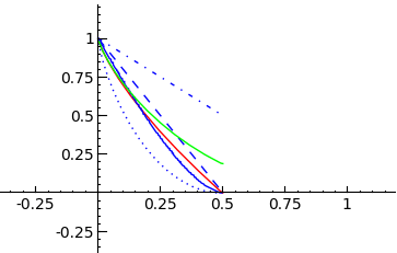
Plot of the Gilbert-Varshamov (dotted), Elias (red), Plotkin (dashed), Singleton (dash-dotted), Hamming (green), and MRRW (stepped) curves using SAGE:

Not a single value of $\alpha_q(x)$ is known for $0<x<{\frac{q-1}{q}}$ !

Goppa’s conjecture: $\alpha_q(x) = 1-H_2(\delta)$ . (In other words, the Gilbert-Varshamov lower bound is actually attained in the case $q=2$ .)

Though my guess is that Goppa’s conjecture is true, it is known (thanks to work of Zink, Vladut and Varshamov) that the q-ary analog of Goppa’s conjecture is false for $q>49$ . On the other hand, we have the following theorem [J].

Theorem: If $B(1.77,p)$ is true for infinitely many primes p with $p\equiv 1\pmod 4$ then Goppa’s conjecture is false.

The rest of this post will be devoted to explaining the notation in this Theorem. The notation $B(c,p)$ means: “For all subsets $S\subset GF(p)$ , $|X_S(GF(p))| \leq c\cdot p$ holds.” The notation $X_S$ means: For each non-empty subset $S\subset GF(p)$ , define the hyperelliptic curve $X_S$ by $y^2=f_S(x)$ , where $f_S(x) = \prod_{a\in S}(x-a)$ .

It may seem strange that a statement about the asymptotic bounds of error-correcting curves is related to the number of points on hyperelliptic curves, but for details see [J]. Unfortunately, it appears much more needs to be known about hyperelliptic curves over finite fields if one is to try to use this connection to prove or disprove Goppa’s conjecture.

References:
[J] D. Joyner, On quadratic residue codes and hyperelliptic curves. Discrete Mathematics & Theoretical Computer Science, Vol 10, No 1 (2008).
[SS] S. Shokranian and M.A. Shokrollahi, Coding theory and bilinear complexity, Scientific Series of the International Bureau, KFA Julich Vol. 21, 1994.

Here’s how the above plot is constructed using SAGE:

sage: f1 = lambda x: gv_bound_asymp(x,2) sage: P1 = plot(f1,0,1/2,linestyle=":") sage: f2 = lambda x: plotkin_bound_asymp(x,2) sage: P2 = plot(f2,0,1/2,linestyle="--") sage: f3 = lambda x: elias_bound_asymp(x,2) sage: P3 = plot(f3,0,1/2,rgbcolor=(1,0,0)) sage: f4 = lambda x: singleton_bound_asymp(x,2) sage: P4 = plot(f4,0,1/2,linestyle="-.") sage: f5 = lambda x: mrrw1_bound_asymp(x,2) sage: P5 = plot(f5,0,1/2,linestyle="steps") sage: f6 = lambda x: hamming_bound_asymp(x,2) sage: P6 = plot(f6,0,1/2,rgbcolor=(0,1,0)) sage: show(P1+P2+P3+P4+P5+P6)

If you are interested in computing what c might be in the above statement B(c,p), the following SAGE code may help.
First, the Python function below will return a random list of elements without repetition, if desired) from an object.

def random_elements(F,n,allow_repetition=True):
    """
    F is a SAGE object for which random_element is a method 
    and having >n elements. For example, a finite field. Here 
    n>1 is an integer. The output is to have no repetitions 
    if allow_repetion=False.
    EXAMPLES:
        sage: p = nth_prime(100)
        sage: K = GF(p)
        sage: random_elements(K,2,allow_repetition=False)
        [336, 186]
    The command random_elements(K,p+1,allow_repetition=False)
    triggers a ValueError.
    """
    if (n>F.order()-2 and allow_repetition==False):
        raise ValueError("Parameters are not well-choosen.")
    L = []
    while len(L)<n:
        c = F.random_element()
        if allow_repetition==False:
            if not(c in L):
                L = L+[c]
        else:
            L = L+[c]
    return L

Next, the SAGE code computes $|X_S(GF(p))|/p$ for a particular choice of the parameters. This gives a lower bound for c.

sage: p = nth_prime(100) sage: K = GF(p) sage: R. = PolynomialRing(K, "x") sage: S = random_elements(K,ZZ((p+1)/2),allow_repetition=False) sage: fS = prod([x - a for a in S]) sage: XS = HyperellipticCurve(fS) sage: RR(len(XS.points())/p) 0.975970425138632
Based on experiments with this code, it appears that for “random” chices of S, and p “large”, the quotient $|X_S(GF(p))|/p$ is very close to 1.

“Circle decoding” of the [7,4,3] Hamming code

Posted on 2008/04/24 by wdjoyner

This is a well-known trick but I’m posting it here since I often have a hard time tracking it down when I need it for an introductory coding theory talk or something. Hopefully someone else will find it amusing too!

Let $F = GF(2)$ and let $C$ be the set of all vectors in the third column below (for simplicity, we omit commas and parentheses, so $0000000$ is written instead of $(0,0,0,0,0,0,0)$ , for example).

The [7,4,3] Hamming code
decimal	binary	Hamming [7,4]
0	0000	0000000
1	0001	0001110
2	0010	0010101
3	0011	0011011
4	0100	0100011
5	0101	0101101
6	0110	0110110
7	0111	0111000
8	1000	1000111
9	1001	1001001
10	1010	1010010
11	1011	1011100
12	1100	1100100
13	1101	1101010
14	1110	1110001
15	1111	1111111

This is a linear code of length 7, dimension 4, and minimum distance 3. It is called the Hamming [7,4,3]-code.
In fact, there is a mapping from $F^4$ to $C$ given by $\phi(x_1,x_2,x_3,x_4)={\bf y}$ , where
${\bf y}= \left( \begin{array}{c} y_1 \\ y_2 \\ y_3 \\ y_4 \\ y_5 \\ y_6 \\ y_7 \end{array} \right) = \left( \begin{array}{cccc} 1&0&0&0 \\ 0&1&0&0 \\ 0&0&1&0 \\ 0&0&0&1 \\ 1&0&1&1 \\ 1&1&0&1 \\ 1&1&1&0 \end{array} \right) \left( \begin{array}{c} x_1 \\ x_2 \\ x_3 \\ x_4 \end{array} \right) \ \pmod{2}$ . Moreover, the matrix $G=\left(\begin{array}{ccccccc} 1&0&0&0&1&1&1 \\ 0&1&0&0&0&1&1 \\ 0&0&1&0&1&0&1 \\ 0&0&0&1&1&1&0 \end{array}\right)$ is a generator matrix.

Now, suppose a codeword $c \in C$ is sent over a noisy channel and denote the received word by ${\bf w}=(w_1,w_2,w_3,w_4,w_5,w_6,w_7)$ . We assume at most 1 error was made.

Put $w_i$ in the region of the Venn diagram above associated to coordinate $i$ in the table below, $i=1,2,...,7$ .
Do parity checks on each of the circles $A$ , $B$ , and $C$ .

Decoding table
parity failure region(s)	error position
none	none
A, B, and C	1
B and C	2
A and C	3
A and B	4
A	5
B	6
C	7

Exercise: Decode ${\bf w} = (0,1,0,0,0,0,1)$ in the binary Hamming code using this algorithm.
(This is solved at the bottom of this column.)

In his 1976 autobiography Adventures of a Mathematician, Stanislaw Ulam [U] poses the following problem:

Someone thinks of a number between one and one million (which is just less than 220). Another person is allowed to ask up to twenty questions, to which the first person is supposed to answer only yes or no. Obviously, the number can be guessed by asking first: Is the number in the first half-million? and then again reduce the reservoir of numbers in the next question by one-half, and so on. Finally, the number is obtained in less than log2(1000000). Now suppose one were allowed to lie once or twice, then how many questions would one need to get the right answer?

We define Ulam’s Problem as follows: Fix integers $M\geq 1$ and $e\geq 0$ . Let Player 1 choose the number from the set of integers $0,1, ...,M$ and Player 2 ask the yes/no questions to deduce the number, to which Player 1 is allowed to lie at most e times. Player 2 must discern which number Player 1 picked with a minimum number of questions with no feedback (in other words, all the questions must be provided at once)

As far as I know, the solution to this version of Ulam’s problem without feedback is still unsolved if e=2. In the case e=1, see [N] and [M]. (Also, [H] is a good survey.)

Player 1 has to convert his number to binary and encode it as a Hamming [7,4,3] codeword. A table containing all 16 codewords is included above for reference. Player 2 then asks seven questions of the form, “Is the i-th bit of your 7-tuple a 1?” Player 1’s answers form the new 7-tuple, $(c_1,c_2,...,c_7)$ , and each coordinate is placed in the corresponding region of the circle. If Player 1 was completely truthful, then the codeword’s parity conditions hold. This means that the 7-tuple generated by Player 2’s questions will match a 7-tuple from the codeword table above. At this point, Player 2 just has to decode his 7-tuple into an integer using the codeword table above to win the game. A single lie, however, will yield a 7-tuple unlike any in the codeword table. If this is the case, Player 2 must error-check the received codeword using the three parity check bits and the decoding table above. In other words, once Player 2 determines the position of the erroneous bit, he corrects it by “flipping its bit”. Decoding the corrected codeword will yield Player 1’s original number.

References

[H] R. Hill, “Searching with lies,” in Surveys in Combinatorics, ed. by P. Rowlinson, London Math Soc, Lecture Notes Series # 218.

[M] J. Montague, “A Solution to Ulam’s Problem with Error-correcting Codes”

[N] I. Niven, “Coding theory applied to a problem of Ulam,” Math Mag 61(1988)275-281.

[U] S. Ulam, Adventures of a mathematician, Scribner and Sons, New York, 1976 .

Solution to exercise using SAGE:

sage: MS = MatrixSpace(GF(2), 4, 7) sage: G = MS([[1,0,0,0,1,1,1],[0,1,0,0,0,1,1],[0,0,1,0,1,0,1],[0,0,0,1,1,1,0]]) sage: C = LinearCode(G) sage: V = VectorSpace(GF(2), 7) sage: w = V([0,1,0,0,0,0,1]) sage: C.decode(w) (0, 1, 0, 0, 0, 1, 1)

In other words, Player picked 4 and lied on the 6th question.

Here is a Sage subtlety:
sage: C = HammingCode(3, GF(2)) sage: C Linear code of length 7, dimension 4 over Finite Field of size 2 sage: V = VectorSpace(GF(2), 7) sage: w = V([0,1,0,0,0,0,1]) sage: C.decode(w) (1, 1, 0, 0, 0, 0, 1)
Why is this decoded word different? Because the Sage Hamming code is distinct (though “equivalent” to) the Hamming code we used in the example above.

Unfortunately, SAGE does not yet do code isomorphisms (at least not as easily as GUAVA), so we use GUAVA’s CodeIsomorphism function, which calls J. Leon’s GPL’s desauto C code function:

gap> C1 := GeneratorMatCode([[1,0,0,1,0,1,0],[0,1,0,1,0,1,1],[0,0,1,1,0,0,1],[0,0,0,0,1,1,1]],GF(2)); a linear [7,4,1..3]1 code defined by generator matrix over GF(2) gap> C2 := GeneratorMatCode([[1,0,0,0,1,1,1],[0,1,0,0,0,1,1],[0,0,1,0,1,0,1],[0,0,0,1,1,1,0]],GF(2)); a linear [7,4,1..3]1 code defined by generator matrix over GF(2) gap> CodeIsomorphism(C1,C2); (2,6,7,3) gap> Display(GeneratorMat(C1)); 1 . . 1 . 1 . . 1 . 1 . 1 1 . . 1 1 . . 1 . . . . 1 1 1 gap> Display(GeneratorMat(C2)); 1 . . . 1 1 1 . 1 . . . 1 1 . . 1 . 1 . 1 . . . 1 1 1 .

Now we see that the permutation (2,6,7,3) sends the “SAGE Hamming code” to the “circle Hamming code”:

sage: H = HammingCode(3, GF(2)) sage: G = MS([[1,0,0,0,1,1,1],[0,1,0,0,0,1,1],[0,0,1,0,1,0,1],[0,0,0,1,1,1,0]]) sage: C = LinearCode(G) sage: C.gen_mat() [1 0 0 0 1 1 1] [0 1 0 0 0 1 1] [0 0 1 0 1 0 1] [0 0 0 1 1 1 0] sage: S7 = SymmetricGroup(7) sage: g = S7([(2,6,7,3)]) sage: H.permuted_code(g) == C True

Yet Another Mathblog

Category Archives: Uncategorized