Introductory example of checking
We may use the field  as the basis for a simple illustrative exercise in the actual procedure of checking. The general of the operations involved will thus be made clear, so far as modus operandi is concerned, and we shall be enabled to discuss more easily the pertinent mathematical details.
It is easy to set up telegraphic codes of high capacity using combinations of four letters each which are not required to be pronounceable. In fact, a sufficiently high capacity may be obtained when only
twenty-three letters of the alphabet are used at all. Hence we can omit any three letters whose Morse equivalents (dot-dash) are most frequently used. Let us suppose that we have before us a code of this kind which employs the letters

and avoids, for reasons stated of for some good reason, the three letters

Suppose that, by prearrangement with telegraphic correspondents, the letters used are paired in
an arbitrary, but fixed, way with the thwenty-three elements of .
Let the pairings be, for instance:

or, in numerical arrangement:

A four-letter group (code word), such as EZRA or XTYP, will indicate a definite entry of a specific page of a definite code volume, several such volumes being perhaps employed in the code. An entry will, in general, be a phrase of sentence, or a group of phrases or sentences, commonly occurring in the class of messages for which the code has been constructed.
Suppose that we have agreed to provide, in our messages, three-letter checks upon groups of twelve letters; in other words, to check in one operation a sequence of three four-letter code words. The twelve letters of the three code words are thus expanded to fifteen; but we send just three telegraphic words — three combinations of five letters, each of which is, in general, unpronounceable.
For illustration, let the first three code words of a message be:

The corresponding sequence of paired elements in is:

This is our operand sequence  :
:

Let us determine the checking matrix  by using as reference matrix
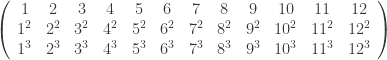
Thus the  are to be

or

Referring to the multiplication table of , we easily compute the .
For the first element  , of the operant sequence , write

For the second element  place a sheet of paper (or a ruler) under the second row
of the multiplication table, and in that row read:  in column ,
  in column ,
  in column . we now have a second line for the tabular scheme:

For the third element  place a sheet of paper (or a ruler) under the third row
of the multiplication table, and in that row read:  in column ,
  in column ,
  in column . We now have the scheme:

The fifth, eighth, and tenth rows of the table will not be used, since
 . The complete scheme is readily found to be:

We have  ,
,  ,
,  .
.
We transmit, of course, the sequence of letters paired, in our system of communications, with the elements of the sequence,
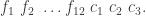
Thus we transmit the sequence of letters: XTYP VZRV HVHH RIF; but we may conveniently agree to transmit it in the arrangement:

or in some other arrangement which employs only three telegraphic words (unpronounceable five letter groups).
We could have used other reference matrices, but we shall not stop to discuss this point. We may remark, however, that if the matrix

had been adopted, the checking elements would have been

and their evaluation would have been accomplished with equal
ease by means of the multiplication table of .

 denote a finite algebraic field with
  elements. It is well-known that, for a given
  is a prime positive integer greater than
  ,
,  is called, according to the terminology of Section 8, Example 2, a ”primary” field. Explicit addition tables, as was noted in section 8, are hardly required in deal ing with primary fields. The most useful of these fields, in telegraphic checking, are probably
  ,
,  , and
, and  . The field
 are positive integers greater than
  may be constructed very easily by algebraic extension of the field
  with the elements (marks)
  , has the tables

 , an equation which is irreducible in
  with marks
 and
and  denote elements of
 . If we label the marks of
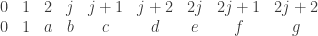
 can be obtained from
  , which is irreducible in
 are elements of
  .
. with the elements (marks)
  , has the tables

 , which is irreducible in the fields
  ,
,  and
and  , we easily obtain the field
  . The marks of
 are elements of
  marks are combined, in the rational operations of
  .
. with the elements (marks)
  , has the tables
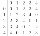

 , we readily obtain the field
  . The marks of
 are elements of
  marks are combined, in the rational operations of

 , and if at least one of the particular elements
  is correctly transmitted, the presence of error will certainly be disclosed. But if exactly three errors are made, affecting presicely the elements
  (
( ) chance of escaping disclosure.
 (
( ) chance of escaping disclosure.


 can be written
  , or
, or  .
.
 can be made quite arbitrarily. But then the values of
  and
and  are then completely determined. There is evidently a

 .
. is the only vanishing determinant of any order in the matrix employed, all other assertions made in (1′) and (2′) are readily justified. This will be made clear in the following sections.
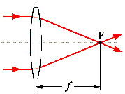
 is the distance from the center of the lens to the principal focal point of the lens. This is illustrated below.
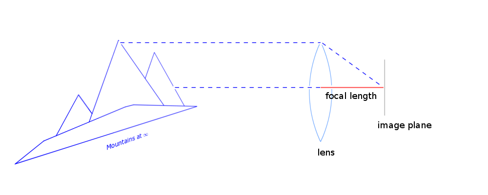
 in front of the lens. This light will meet the sensor plane but its image in the photo, depending on the value of
  .
. .
. mm. To focus an object 1 m away (
 mm), we solve for
  . Therefore, the lens must be moved 2.6 mm further away from the image plane, to
  mm.
mm.
 is an opening which is half the focal length, so if
  (read “the f-stop is N”, where
  ) then
  is called the f-number or f-stop. Two apertures (or f-stops) are said to differ by a full stop if they differ by a factor of
  . Usually the stop numbers fall into the sequence


 be a prime power such that
  . Note that this implies that the unique finite field of order
  , has a square root of
  . Now let
  and
and
 if and only if
  . By definition
  is the
  (with multiplicity
  (both with multiplicity
  , where
  has order
  .
. ” above; I was having trouble rendering it in html.) Below is an example.
 .
. :
:
 (about 82 billion) different orders that the spider can put on shoes and socks.
You must be logged in to post a comment.