If you were a math textbook …

Posted on 2013/08/01 by wdjoyner

If I were a Springer-Verlag Graduate Text in Mathematics, I would be David Eisenbud’s Commutative Algebra with a view towards Algebraic Geometry.

I am an attempt to write on commutative algebra in a way that includes the geometric ideas that played a great role in its formation; with a view, in short, towards Algebraic Geometry. I cover the material that graduate students studying Algebraic Geometry – and in particular those studying the book Algebraic Geometry by Robin Hartshorne – should know. The reader should have had one year of basic graduate algebra.

Which Springer GTM would you be? The Springer GTM Test

A 1932 memorandum on rum-runner’s cryptosystems

Posted on 2013/07/12 by wdjoyner

During the prohibition era, organized crime made phenomenal amounts of money through illegal smuggling. Eventually, their messages were enciphered. By the late 1920s and early 1930s, these cryptosystems became rather sophisticated. Here is a memorandum form Elizebeth Friedman to CMDR Gorman in January or 1932 which gives an indication of this sophistication.

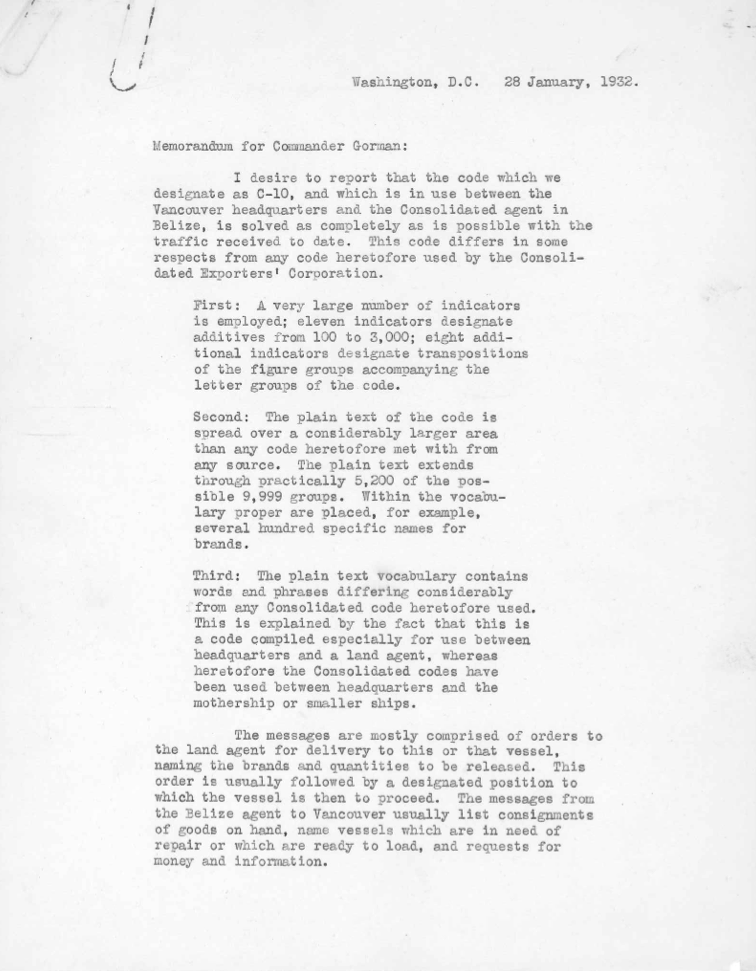
Many thanks to the George C. Marshall Foundation, Lexington, Virginia, for providing this reproduction!

A 1926 message from “I Am Alone”

Posted on 2013/07/04 by wdjoyner

The I Am Alone, flying a Canadian flag, was a rumrunner sunk by Coast Guard patrol boats in the Gulf of Mexico in March, 1929. The USCG knew that the ship was not a Canadian owned-and-controlled vessel but the proof went down to the bottom of the ocean when it was sunk. The Canadian Government sued the United States for $365,000 and the ensuing legal battle brought world-wide attention. Elizebeth Friedman decoded the messages transmitted by the I Am Alone, and those messages proved that the boat was, in fact, not a Canadian owned-and-controlled vessel. The case actually went to a Commission, whose final report was issued in 1935. They found, thanks in part to Elizebeth Friedman, that the owners and controllers of the vessel were not Canadian and used the boat primarily for illegal purposes.

The image below is a scan of an intercepted message, dated 1926-02-15, from the I Am Alone.

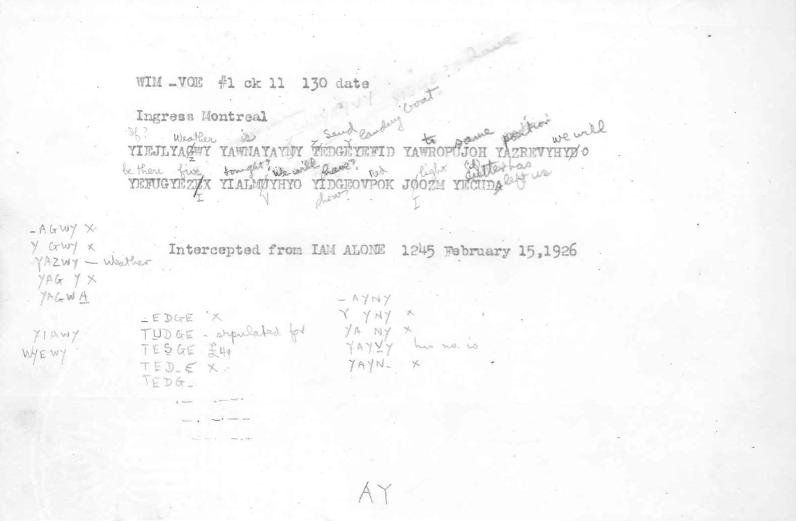
The writing is that of EF and you can make out her (mostly) deciphered message.

For more information, see, for example,
“All Necessary Force”: The Coast Guard And The Sinking of the Rum Runner “I’m Alone” by Joseph Anthony Ricci, 2011, or
“Listening to the rumrunners” by David Mowry, 2001.

The above image is courtesy of the Elizebeth S. Friedman Collection at the George C. Marshall Foundation, Lexington, Virginia. (If you make use of the image, please acknowledge the Marshall Foundation.)

Lester Hill’s “The checking of the accuracy …”, part 10

Posted on 2013/06/02 by wdjoyner

Construction of finite fields for use in checking

Let $F_\Gamma$ denote a finite algebraic field with $\Gamma$ elements. It is well-known that, for a given $\Gamma$ , all fields $F_\Gamma$ are “simply isomorphic”, and therewith, for our purposes, identical. We shall consequently refer, without restraint, to ”the field $F_\Gamma$ .”

If $p$ is a prime positive integer greater than $1$ , $F_p$ is called, according to the terminology of Section 8, Example 2, a ”primary” field. Explicit addition tables, as was noted in section 8, are hardly required in deal ing with primary fields. The most useful of these fields, in telegraphic checking, are probably $F_{23}$ , $F_{29}$ , $F_{31}$ , and $F_{101}$ . The field $F_{101}$ will be considered in detail in what follows.

The number of elements in a non-primary finite algebraic field
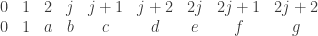
is a power of a prime. If we have

$q=p^k$
where $p$ and $k$ are positive integers greater than $1$ , and $p$ is prime, the non-primary field $F_q$ may be constructed very easily by algebraic extension of the field $F_p$ . Explicit addition table is needed when working with a non-primary field. Otherwise, checking operations are exactly the same as in primary fields.

Example: The field $F_3$ with the elements (marks) $0,1,2$ , has the tables

$\begin{array}{r|*{3}{r}} \multicolumn{1}{c|} +&0&1&2\\\hline {}0&0&1&2\\ {}1&1&2&0\\ {}2&2&0&1\\ \end{array}$
$\begin{array}{r|*{3}{r}} \multicolumn{1}{c|} \cdot &0&1&2\\\hline {}0&0&0&0\\ {}1&0&1&2\\ {}2&0&2&1\\ \end{array}$

By adjoining a root of the equation $x^2=2$ , an equation which is irreducible in $F_3$ , we easily obtain the field $F_9$ with marks

$\alpha j+\beta$
where $\alpha$ and $\beta$ denote elements of $F_3$ . The marks of $F_9$ are thus

$0,1,2,j,j+1,j+2,2j,2j+1,2j+2.$
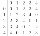
These marks (elements) are combined, in the rational field operations of $F_9$ , according to the reduction formula $j^2=2$ . If we label the marks of $F_9$ as follows

$\begin{array}{ccccccccc} 0 & 1 & 2 & j & j+1& j+2& 2j& 2j+1& 2j+2\\ 0 & 1 & a & b & c & d & e & f & g\\ \end{array}$
the addition and multiplication tables of the field are given as in
Section 8, Example 1.

In a like manner, $F_{27}$ can be obtained from $F_3$ by adjunction of a root of the equation $x^3=x+1$ , which is irreducible in $F_3$ and $F_9$ . The marks (elements) of $F_{27}$ are

$\alpha j^2+\beta j+\gamma,$
where $\alpha,\beta,\gamma$ are elements of $F_3$ . They are combined, in the rational operations of $F_{27}$ according to the reduction formula $j^3=j+1$ .

Example: The field $F_2$ with the elements (marks) $0,1$ , has the tables

$\begin{array}{r|*{2}{r}} \multicolumn{1}{c|} + &0&1\\ \hline {}0&0&1\\ {}1&1&0\\ \end{array}$
$\begin{array}{r|*{2}{r}} \multicolumn{1}{c|} \cdot &0&1\\ \hline {}0&0&0\\ {}1&0&1\\ \end{array}$

By adjunction of a root of the equation $x^5=x^2+1$ , which is irreducible in the fields $F_2$ , $F_4$ , $F_8$ and $F_{16}$ , we easily obtain the field $F_{32}$ . The marks of $F_{32}$ are

$\alpha j^4+\beta j^3+\gamma j^2+\delta j+\epsilon,$
where $\alpha,\beta,\gamma, \delta,\epsilon$ are elements of $F_2$ ; and these $32$ marks are combined, in the rational operations of $F_{32}$ , according to the reduction formula $j^5=j^2+1$ .

Example: The field $F_5$ with the elements (marks) $0,1,2,3,4$ , has the tables

$\begin{array}{r|*{5}{r}} \multicolumn{1}{c|} +&0&1&2&3&4\\\hline {}0&0&1&2&3&4\\ {}1&1&2&3&4&0\\ {}2&2&3&4&0&1\\ {}3&3&4&0&1&2\\ {}4&4&0&1&2&3\\ \end{array}$
$\begin{array}{r|*{5}{r}} \multicolumn{1}{c|} \cdot &0&1&2&3&4\\\hline {}0&0&0&0&0&0\\ {}1&0&1&2&3&4\\ {}2&0&2&4&1&3\\ {}3&0&3&1&4&2\\ {}4&0&4&3&2&1\\ \end{array}$

By adjoining a root of the equation $x^2=2$ , which is irreducible in $F_{5}$ , we readily obtain the field $F_{25}$ . The marks of $F_{25}$ are

$\alpha j+\beta ,$
where $\alpha,\beta$ are elements of $F_5$ ; and these $25$ marks are combined, in the rational operations of $F_{25}$ , according to the reduction formula $j^2=2$ .

Of the non-primary fields, $F_{25}$ , $F_{27}$ , $F_{32}$ are probably those which are most amenable to practical application in telegraphic checking.

mathematics problem 155

Posted on 2013/06/02 by wdjoyner

A colleague Bill Wardlaw (March 3, 1936-January 2, 2013) used to create a “Problem of the Week” for his students, giving a prize of a cookie if they could solve it. Here is one of them.

Mathematics Problem, #155

We can represent a triangle with sides of length a, b, c by the ordered triple (a, b, c). Changing the order of the sides doesn’t change the triangle, so (a, b, c), (b, a, c), (b, c, a), (c, b, a), (c, a, b), and (a, c, b) all represent the same triangle. To avoid confusion, let’s agree to write (a, b, c) with a < b < c. We say that a triangle <I (a, b, c) is integral if a, b, and c are integers. How many integral triangles are there with longest side less than or equal to 100 ?

Mathematics Problem 154

Posted on 2013/06/02 by wdjoyner

A colleague Bill Wardlaw (March 3, 1936-January 2, 2013) used to create a “Problem of the Week” for his students, giving a prize of a cookie if they could solve it. Here is one of them.

Mathematics Problem, #154

Find the volume of the intersection of three cylinders, each of radius a, which are centered on the x-axis, the y-axis, and the z-axis. That is, find the volume of the three dimensional region

E = {(x,y,z) | x² + y² < a², y² + z² < a², z² + x² < a²}.

Lester Hill’s “The checking of the accuracy …”, part 9

Posted on 2013/05/27 by wdjoyner

We may inquire into the possibility of undisclosed errors occurring in the transmittal of the sequence:

$\begin{array}{ccccccccccccccc} f_1 & f_2 & f_3 & f_4 & f_5 & f_6 & f_7 & f_8 & f_9 & f_{10} & f_{11} & f_{12} & c_1 & c_2 & c_3 \\ 5 & 17 & 13 & 21 & 0 & 8 & 6 & 0 & 11 & 0 & 11 & 11 & 6 & 15 & 2 \\ X & T & Y & P & V & Z & R & V & H & V & H & H & R & I & F \\ \end{array}$

Invoking the theorem established in sections 4 and 5, and formulated at the close of section 5, we may assert:

(1) If not more than three errors are made in transmitting the fifteen letters of the sequence, and if the errors made affect the $f_i$ only, the $c_j$ being correctly transmitted, then the presence of error is certain to be disclosed.
(2) If not more than three errors are made, all told, but at least three of them affect the $f_i$ , then the presence of error will enjoy only a

$1-{\rm in}-22^3\ \ \ \ \ (1-{\rm in}-10648)$
chance of escaping disclosure.

These assertions result at once from the theorem referred to. But a closer study of the reference matrix employed in this example permits us to replace them by the following more satisfactory statements:

(1′)
If errors occur in not more than three of the fifteen elements of the sequence $f_1f_2\dots f_{12}c_1 c_2 c_3$ , and if at least one of the particular elements $f_{11}f_{12}c_2$ is correctly transmitted, the presence of error will certainly be disclosed. But if exactly three errors are made, affecting presicely the elements $f_{11}f_{12}c_2$ , the presence of error will enjoy a $1$ -in- $22^2$ ( $1$ -in- $484$ ) chance of escaping disclosure.
(2′)
If more than three errors are made, then whatever the distribution of errors among the fifteen elements of the sequence, the presence of error will enjoy only a
$1$ -in- $22^3$ ( $1$ -in- $10648$ ) chance of escaping disclosure.

Assertions of this kind will be carefully established below, when a more important finite field is under consideration. The argument then made will be applicable in the case of any finite field. But it is worthwhile here to look more carefully into the exceptional distribution of errors which is italicized in (1′). This will help us note any weakness that ought to be avoided in the construction of reference matrices.

Suppose that exactly three errors are made, affecting precisely $f_{11}f_{12}c_2$ . If the mutilated message is to check up, and the errors to escape disclosure, we must have (for error notations, see sections 4,5):

$11\epsilon_{11}+12\epsilon_{12}=0,\ \ \ 11^2\epsilon_{11}+12^2\epsilon_{12}=\delta_2,\ \ \ 11^3\epsilon_{11}+12^3\epsilon_{12}=0.$
These equations may be written:

$11\epsilon_{11}+12\epsilon_{12}=0,\ \ \ 6\epsilon_{11}+6\epsilon_{12}=\delta_2,\ \ \ 20\epsilon_{11}+3\epsilon_{12}=0.$
But $11\epsilon_{11}=-12\epsilon_{12}$ can be written $11\epsilon_{11}=11\epsilon_{12}$ , or $\epsilon_{11}=\epsilon_{12}$ .
Etc. In this way, we find that the errors can escape disclosure if and only if

$\epsilon_{11}=\epsilon_{12},\ \ \ {\rm and}\ \ \ \delta_{2}=12\epsilon_{11}.$
The error $\epsilon_{11}$ can be made quite arbitrarily. But then the values of $\epsilon_{12}$ and $\delta_2$ are then completely determined. There is evidently a $1$ -in- $484$ chance – and no more – that the errors will fall out just right.

The trouble arises from the vanishing, in our reference matrix, of the two-rowed
determinant

$\big{|} \begin{array}{cc} 11 & 12 \\ 11^3 & 12^3 \end{array} \big{|} .$
Note that

$\big{|} \begin{array}{cc} 11 & 12 \\ 11^3 & 12^3 \end{array} \big{|} = 11\cdot 12\cdot \big{|} \begin{array}{cc} 1 & 1 \\ 11^2 & 12^2 \end{array} \big{|} = 17 \big{|} \begin{array}{cc} 1 & 1 \\ 11^2 & 12^2 \end{array} \big{|} =0,$
since $11^2=12^2$ .

From the fact that $\big{|} \begin{array}{cc} 11 & 12 \\ 11^3 & 12^3 \end{array} \big{|}$ is the only vanishing determinant of any order in the matrix employed, all other assertions made in (1′) and (2′) are readily justified. This will be made clear in the following sections.

It will be advantageous, as shown more completely in subsequent sections, to employ reference matrices which contain the smallest possible number of vanishing determinants of any orders.

Mathematical notes on Depth of Field

Posted on 2013/05/27 by wdjoyner

There are a million blog posts on photography depth of field (DOF). This one makes a million and one! If writing this will help me, and hopefully someone else, understand it better, it will be worth it.

We assume that a typical camera lens is fixed in space and represents the properties of a “thin convex lens in air”. We say an object, such as a distant mountain, is at infinity if light from it enters the lens along a ray perpendicular, or nearly perpendicular, to the lens plane. The principal focal point is that point behind the lens that an object at infinity (on the axis of the lens) focuses to. 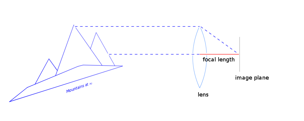The focal length $f$ is the distance from the center of the lens to the principal focal point of the lens. This is illustrated below.

mountains “at infinity” with respect to lens, created using GIMP and Sage

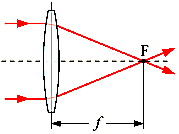
Focal length for a convex lens (source: Wikipedia)

Define the object plane to be the plane of the object you are photographing parallel to the plane of the lens) and want to look sharp in your photo. (Again, the object is assumed to be on the axis of the lens.) The light from the object converges behind the lens to a small region called the image. The image plane is a plane (parallel to the lens) which intersects this image region. You want the plane of the digital sensor (or camera film) to be at or very near the image plane, or else the photo will not have the object in focus.

We assume that the camera is a projective transformation from the plane of the object to the plane of the digital sensor. In other words, we assume that the camera has the property that if it focuses on a (stright) line or circle then it captures a line or circle on the film or digital sensor. (Of course, in reality, the lens imperfections and the light diffraction have an effect, but this hypothesis is nearly true in many cases.)

Consider an object at infinity (say, some distant mountains) in the plane of the plane of your lens. Suppose your camera’s digital sensor is located in the same plane as the image plane, so that the mountains will be in focus in your camera. The distance from the lens to the sensor plane is the focal length $f$ . Consider the light entering your lens from a small disk (also on the axis of the lens) at a distance $u$ in front of the lens. This light will meet the sensor plane but its image in the photo, depending on the value of $u$ , may or may not be in focus. If the disk is relatively small in diameter then its blurred image on the photo is sometimes called a circle of confusion. Concretely speaking, the circle of confusion measures the maximum diameter on an 8′′ × 10′′ photo for which there is an acceptable blur in the image of the disk. Suppose now that the distance between the lens and sensor plane (say that the lens, along with the disk in front of it, are fixed but the sensor plane is translated backwards) is increased until this small disk is in focus in the photo. Call this new distance between the lens and the sensor plane $v$ .

Lemma 1. The focal length $f$ , the distance from the lens to the object to photograph $u$ , and the distance from lens to the image focus plane $v$ are then related by the lens equation $\frac{1}{u}+\frac{1}{v}=\frac{1}{f}$ .

Example: As $v$ is decreased, $u$ must be increased. For example, consider a normal lens for a 35 mm camera with a focal length of $f = 50$ mm. To focus an object 1 m away ( $u = 1000$ mm), we solve for $v = \frac{1}{\frac{1}{f}-\frac{1}{u}} = 1000/19 = 52.63...$ . Therefore, the lens must be moved 2.6 mm further away from the image plane, to $v = 52.6$ mm.

The depth of field (DOF) is the portion of a scene that appears sharp in the image. More precisely, it is the area near the object plane in which the circles of confusion are acceptably small (where “acceptably small” has some precise pre-defined meaning, e.g., 0.2mm for a photo blown up to an 8′′ × 10′′ print). Although a lens can precisely focus at only one distance, the decrease in sharpness is gradual on either side of the focused distance, so that within the DOF, the unsharpness is imperceptible under normal viewing conditions. See the image below for an example of an image with a “small” (or “short”) DOF.

snowflake, small DOF example

The lens aperture is the circular opening in the lens allowing light to pass through. The actual diameter of opening is called the effective aperture. By convention, the aperture is measured as a quotient relative to the focal length $f$ . For example, the aperture $f/2$ is an opening which is half the focal length, so if $f = 50$ mm then the effective aperture would be a disc of diameter 25mm. In general, if the aperture is $f/N$ (read “the f-stop is N”, where $N \geq 1$ ) then $N$ is called the f-number or f-stop. Two apertures (or f-stops) are said to differ by a full stop if they differ by a factor of $\sqrt{2}$ . Usually the stop numbers fall into the sequence

$1, \sqrt{2}, 2, 2\sqrt{2}, 4, 4\sqrt{2}, 8, 8\sqrt{2}, 16, 16\sqrt{2}, 32, 32\sqrt{2}, ...,$

which might be rounded up or down to

$1, 1.4, 2, 2.8, 4, 5.6, 8, 11, 16, 22, 32, 45, ....$

The larger f-stop is, the smaller the aperture.

An aperture slide card for an old-fashioned camera.

For more details, see for example:

Jeff Conrad, Depth of field in depth, preprint 2006. Available at: http://www.largeformatphotography.info/.
L. Evens, View camera geometry, preprint, 2008.
R. E. Wheeler, Notes on view camera geometry, preprint, 2003.

Paley graphs in Sage

Posted on 2013/03/06 by wdjoyner

Let $q$ be a prime power such that $q\equiv 1 \pmod 4$ . Note that this implies that the unique finite field of order $q$ , $GF(q)$ , has a square root of $-1$ . Now let $V=GF(q)$ and

$E = \{(a,b)\in V\times V\ |\ a-b\in GF(q)^2\}.$
By hypothesis, $(a,b)\in E$ if and only if $(b,a)\in E$ . By definition $G = (V, E)$ is the Paley graph of order $q$ .

Paley was a brilliant mathematician who died tragically at the age of 26. Paley graphs are one of the many spin-offs of his work. The following facts are known about them.

The eigenvalues of Paley graphs are $\frac{q-1}{2}$ (with multiplicity $1$ ) and
$\frac{-1 \pm \sqrt{q}}{2}$ (both with multiplicity $\frac{q-1}{2}$ ).
It is known that a Paley graph is a Ramanujan graph.
It is known that the family of Paley graphs of prime order is a vertex expander graph family.
If $q=p^r$ , where $p$ is prime, then $Aut(G)$ has order $rq(q-1)/2$ .

Here is Sage code for the Paley graph (thanks to Chris Godsil, see [GB]):

def Paley(q):
    K = GF(q)
    return Graph([K, lambda i,j: i != j and (i-j).is_square()])

(Replace “K” by “ $K.\langle a\rangle$ ” above; I was having trouble rendering it in html.) Below is an example.

sage: X = Paley(13)
sage: X.vertices()
[0, 1, 2, 3, 4, 5, 6, 7, 8, 9, 10, 11, 12]
sage: X.is_vertex_transitive()
True
sage: X.degree_sequence()
[6, 6, 6, 6, 6, 6, 6, 6, 6, 6, 6, 6, 6]
sage: X.spectrum()
[6, 1.302775637731995?, 1.302775637731995?, 1.302775637731995?,
1.302775637731995?, 1.302775637731995?, 1.302775637731995?,
-2.302775637731995?, -2.302775637731995?, -2.302775637731995?,
-2.302775637731995?, -2.302775637731995?, -2.302775637731995?]
sage: G = X.automorphism_group()
sage: G.cardinality()
78

We see that this Paley graph is regular of degree $6$ , it has only three distinct eigenvalues, and its automorphism group is order $13\cdot 12/2 = 78$ .

Here is an animation of this Paley graph:

The frames in this animation were constructed one-at-a-time by deleting an edge and plotting the new graph.

Here is an animation of the Paley graph of order $17$ :

The frames in this animation were constructed using a Python script:

X = Paley(17)
E = X.edges()
N = len(E)
EC = X.eulerian_circuit()
for i in range(N):
    X.plot(layout="circular", graph_border=True, dpi=150).save(filename="paley-graph_"+str(int("1000")+int("%s"%i))+".png")
    X.delete_edge(EC[i])
X.plot(layout="circular", graph_border=True, dpi=150).save(filename="paley-graph_"+str(int("1000")+int("%s"%N))+".png")

Instead of removing the frames “by hand” they are removed according to their occurrence in a Eulerian circuit of the graph.

Here is an animation of the Paley graph of order $29$ :

[GB] Chris Godsil and Rob Beezer, Explorations in Algebraic Graph Theory with Sage, 2012, in preparation.

Mathematics Problem, #120

Posted on 2013/03/06 by wdjoyner

A colleague Bill Wardlaw (March 3, 1936-January 2, 2013) used to create a “Problem of the Week” for his students, giving a prize of a cookie if they could solve it. Here is one of them.

Mathematics Problem, #120

A calculus 1 student Joe asks another student Bob “Is the following expression correct?” and writes

$f'(x^3)=3x^2$
on the blackboard. Bob replies, “Well, it could be, but I don’t think that is what you mean.”

Find a function that makes what Joe said correct.

Solution to #119:
There are $(16!)/(2^8)$ (about 82 billion) different orders that the spider can put on shoes and socks.