More odd examples of p-ary bent functions

In an earlier post I discussed bent functions $f:GF(3)^2\to GF(3)$ . In this post, I’d like to give some more examples, based on a recent paper with Caroline Melles, Charles Celerier, David Phillips, and Steven Walsh, based on computations using Sage/pythpn programs I wrote with Charles Celerier.

We start with any function $f:GF(p)^n\to GF(p)$ . The Cayley graph of $f$ is defined to be the edge-weighted digraph

$\Gamma_f = (GF(p)^n, E_f ),$
whose vertex set is $V=V(\Gamma_f)=GF(p)^n$ and the set of edges is defined by

$E_f =\{(u,v) \in GF(p)^n\ |\ f(u-v)\not= 0\},$
where the edge $(u,v)\in E_f$ has weight $f(u-v)$ . However, if $f$ is even then we can (and do) regard $\Gamma_f$ as an edge-weighted (undirected) graph.

We assume, unless stated otherwise, that $f$ is even.

For each $u\in V$ , define

$N(u)=N_{\Gamma_f}(u)$ to be the set of all neighbors of $u$ in $\Gamma_f$ ,
$N(u,a)=N_{\Gamma_f}(u,a)$ to be the set of all neighbors $v$ of $u$ in $\Gamma_f$ for which the edge $(u,v)\in E_f$ has weight $a$ (for each $a\in GF(p)^\times = GF(p)-\{0\}$ ),
$N(u,0)=N_{\Gamma_f}(u,0)$ to be the set of all non-neighbors $v$ of $u$ in $\Gamma_f$ (i.e., we have $(u,v)\notin E_f$ ),
the support of $f$ is
${\rm supp}(f)=\{v\in V\ |\ f(v)\not=0\}$

Let $\Gamma$ be a connected edge-weighted graph which is regular as a simple (unweighted) graph. The graph $\Gamma$ is called strongly regular with parameters $v$ , $k=(k_a)_{a\in W}$ , $\lambda=(\lambda_a)_{a\in W^3}$ , $\mu=(\mu_a)_{a\in W^2}$ , denoted $SRG_{W}(v,k,\lambda,\mu)$ , if it consists of $v$ vertices such that, for each $a=(a_1,a_2)\in W^2$

$|N(u_1,a_1) \cap N(u_2,a_2)| = \left\{ \begin{array}{ll} k_{a}, & u_1=u_2,\\ \lambda_{a_1,a_2,a_3}, & u_1\in N(u_2,a_3),\ u_1\not= u_2,\\ \mu_{a}, &u_1\notin N(u_2),\ u_1\not= u_2,\\ \end{array} \right.$
where $k$ , $\lambda$ , $\mu$ are as above. Here, $W= GF(p)$ is the set of weights, including $0$ (recall an “edge” has weight $0$ if the vertices are not neighbors).

This example is intended to illustrate the bent function $b_8$ listed in the table below
$\begin{array}{c|ccccccccc} GF(3)^2 & (0, 0) & (1, 0) & (2, 0) & (0, 1) & (1, 1) & (2, 1) & (0, 2) & (1, 2) & (2, 2) \\ \hline b_8 & 0 & 2 & 2 & 0 & 0 & 1 & 0 & 1 & 0 \\ \end{array}$

Consider the finite field
$GF(9) = GF(3)[x]/(x^2+1) = \{0,1,2,x,x+1,x+2,2x,2x+1,2x+2\}.$
The set of non-zero quadratic residues is given by
$D = \{1,2,x,2x\}.$
Let $\Gamma$ be the graph whose vertices are $GF(9)$ and whose edges $e=(a,b)$ are those pairs for which $a-b\in D$ .

The graph looks like the Cayley graph for $b_8$ in the Figure below

Bent function b_8 on GF(3)^2

except

$8\to 0, 0\to 2x+2, 1\to 2x+1, 2\to 2x,$
$3\to x+2, 4\to x+1, 5\to x, 6\to 2, 7\to 1, 8\to 0.$
This is a strongly regular graph with parameters $(9,4,1,2)$ .

$\begin{array}{c|ccccccccc} v & 0 & 1 & 2 & 3 & 4 & 5 & 6 & 7 & 8 \\ \hline N(v,0) & 3,4,6,8 & 4,5,6,7 & 3,5,7,8 & 0,2,6,7 & 0,1,7,8 & 1,2,6,8 & 0,1,3,5 & 1,2,3,4 & 0,2,4,5 \\ N(v,1) & 5,7 & 3,8 & 4,6 & 1,8 & 2,6 & 0,7 & 2,4 & 0,5 & 1,3 \\ N(v,2) & 1,2 & 0,2 & 0,1 & 4,5 & 3,5 & 3,4 & 7,8 & 6,8 & 6,7 \\ \end{array}$

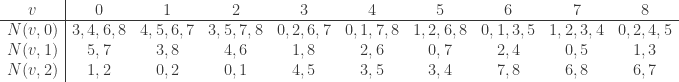
The axioms of an edge-weighted strongly regular graph can be directly verified using this table.

Let $S$ be a finite set and let $R_0, R_1, \dots, R_s$ denote binary relations on $S$ (subsets of $S\times S$ ). The dual of a relation $R$ is the set

$R^* = \{(x,y)\in S\times S\ |\ (y,x)\in R\}.$
Assume $R_0=\Delta_S= \{ (x,x)\in S\times S\ |\ x\in S\}$ . We say $(S,R_0,R_1,\dots,R_s)$ is an $s$ -class association scheme on $S$ if the following properties hold.

We have a disjoint union
$S\times S = R_0\cup R_1\cup \dots \cup R_s,$
with $R_i\cap R_j=\emptyset$ for all $i\not= j$.
For each $i$ there is a $j$ such that $R_i^*=R_j$ (and if $R_i^*=R_i$ for all $i$ then we say the association scheme is symmetric).
For all $i,j$ and all $(x,y)\in S\times S$ , define
$p_{ij}(x,y) = |\{z\in S\ |\ (x,z)\in R_i, (z,y)\in R_j\}|.$
For each $k$ , and for all $x,y\in R_k$ , the integer $p_{ij}(x,y)$ is a constant, denoted $p_{ij}^k$ .

These constants $p_{ij}^k$ are called the intersection numbers of the association scheme.

For this example of $b_8$ , we compute the adjacency matrix associated to the members $R_1$ and $R_2$ of the association scheme $(G,R_0,R_1,R_2,R_3)$ , where $G = GF(3)^2$ ,

$R_i = \{(g,h)\in G\times G\ |\ gh^{-1} \in D_i\},\ \ \ \ \ i=1,2,$
and $D_i = f^{-1}(i)$ .

Consider the following Sage computation:

sage: attach "/home/wdj/sagefiles/hadamard_transform2b.sage"
sage: FF = GF(3)
sage: V = FF^2
sage: Vlist = V.list()
sage: flist = [0,2,2,0,0,1,0,1,0]
sage: f = lambda x: GF(3)(flist[Vlist.index(x)])
sage: F = matrix(ZZ, [[f(x-y) for x in V] for y in V])
sage: F  ## weighted adjacency matrix
[0 2 2 0 0 1 0 1 0]
[2 0 2 1 0 0 0 0 1]
[2 2 0 0 1 0 1 0 0]
[0 1 0 0 2 2 0 0 1]
[0 0 1 2 0 2 1 0 0]
[1 0 0 2 2 0 0 1 0]
[0 0 1 0 1 0 0 2 2]
[1 0 0 0 0 1 2 0 2]
[0 1 0 1 0 0 2 2 0]
sage: eval1 = lambda x: int((x==1))
sage: eval2 = lambda x: int((x==2))
sage: F1 = matrix(ZZ, [[eval1(f(x-y)) for x in V] for y in V])
sage: F1
[0 0 0 0 0 1 0 1 0]
[0 0 0 1 0 0 0 0 1]
[0 0 0 0 1 0 1 0 0]
[0 1 0 0 0 0 0 0 1]
[0 0 1 0 0 0 1 0 0]
[1 0 0 0 0 0 0 1 0]
[0 0 1 0 1 0 0 0 0]
[1 0 0 0 0 1 0 0 0]
[0 1 0 1 0 0 0 0 0]
sage: F2 = matrix(ZZ, [[eval2(f(x-y)) for x in V] for y in V])
sage: F2
[0 1 1 0 0 0 0 0 0]
[1 0 1 0 0 0 0 0 0]
[1 1 0 0 0 0 0 0 0]
[0 0 0 0 1 1 0 0 0]
[0 0 0 1 0 1 0 0 0]
[0 0 0 1 1 0 0 0 0]
[0 0 0 0 0 0 0 1 1]
[0 0 0 0 0 0 1 0 1]
[0 0 0 0 0 0 1 1 0]
sage: F1*F2-F2*F1 == 0
True
sage: delta = lambda x: int((x[0]==x[1]))
sage: F3 = matrix(ZZ, [[(eval0(f(x-y))+delta([x,y]))%2 for x in V] for y in V])
sage: F3
[0 0 0 1 1 0 1 0 1]
[0 0 0 0 1 1 1 1 0]
[0 0 0 1 0 1 0 1 1]
[1 0 1 0 0 0 1 1 0]
[1 1 0 0 0 0 0 1 1]
[0 1 1 0 0 0 1 0 1]
[1 1 0 1 0 1 0 0 0]
[0 1 1 1 1 0 0 0 0]
[1 0 1 0 1 1 0 0 0]
sage: F3*F2-F2*F3==0
True
sage: F3*F1-F1*F3==0
True
sage: F0 = matrix(ZZ, [[delta([x,y]) for x in V] for y in V])
sage: F0
[1 0 0 0 0 0 0 0 0]
[0 1 0 0 0 0 0 0 0]
[0 0 1 0 0 0 0 0 0]
[0 0 0 1 0 0 0 0 0]
[0 0 0 0 1 0 0 0 0]
[0 0 0 0 0 1 0 0 0]
[0 0 0 0 0 0 1 0 0]
[0 0 0 0 0 0 0 1 0]
[0 0 0 0 0 0 0 0 1]
sage: F1*F3 == 2*F2 + F3
True

The Sage computation above tells us that the adjacency matrix of $R_1$ is

$A_1 = \left(\begin{array}{rrrrrrrrr} 0 & 0 & 0 & 0 & 0 & 1 & 0 & 1 & 0 \\ 0 & 0 & 0 & 1 & 0 & 0 & 0 & 0 & 1 \\ 0 & 0 & 0 & 0 & 1 & 0 & 1 & 0 & 0 \\ 0 & 1 & 0 & 0 & 0 & 0 & 0 & 0 & 1 \\ 0 & 0 & 1 & 0 & 0 & 0 & 1 & 0 & 0 \\ 1 & 0 & 0 & 0 & 0 & 0 & 0 & 1 & 0 \\ 0 & 0 & 1 & 0 & 1 & 0 & 0 & 0 & 0 \\ 1 & 0 & 0 & 0 & 0 & 1 & 0 & 0 & 0 \\ 0 & 1 & 0 & 1 & 0 & 0 & 0 & 0 & 0 \end{array}\right),$
the adjacency matrix of $R_2$ is

$A_2 = \left(\begin{array}{rrrrrrrrr} 0 & 1 & 1 & 0 & 0 & 0 & 0 & 0 & 0 \\ 1 & 0 & 1 & 0 & 0 & 0 & 0 & 0 & 0 \\ 1 & 1 & 0 & 0 & 0 & 0 & 0 & 0 & 0 \\ 0 & 0 & 0 & 0 & 1 & 1 & 0 & 0 & 0 \\ 0 & 0 & 0 & 1 & 0 & 1 & 0 & 0 & 0 \\ 0 & 0 & 0 & 1 & 1 & 0 & 0 & 0 & 0 \\ 0 & 0 & 0 & 0 & 0 & 0 & 0 & 1 & 1 \\ 0 & 0 & 0 & 0 & 0 & 0 & 1 & 0 & 1 \\ 0 & 0 & 0 & 0 & 0 & 0 & 1 & 1 & 0 \end{array}\right),$
and the adjacency matrix of $R_3$ is

$A_3 = \left(\begin{array}{rrrrrrrrr} 0 & 0 & 0 & 1 & 1 & 0 & 1 & 0 & 1 \\ 0 & 0 & 0 & 0 & 1 & 1 & 1 & 1 & 0 \\ 0 & 0 & 0 & 1 & 0 & 1 & 0 & 1 & 1 \\ 1 & 0 & 1 & 0 & 0 & 0 & 1 & 1 & 0 \\ 1 & 1 & 0 & 0 & 0 & 0 & 0 & 1 & 1 \\ 0 & 1 & 1 & 0 & 0 & 0 & 1 & 0 & 1 \\ 1 & 1 & 0 & 1 & 0 & 1 & 0 & 0 & 0 \\ 0 & 1 & 1 & 1 & 1 & 0 & 0 & 0 & 0 \\ 1 & 0 & 1 & 0 & 1 & 1 & 0 & 0 & 0 \end{array}\right)$
Of course, the adjacency matrix of $R_0$ is the identity matrix. In the above computation, Sage has also verified that they commute and satisfy

$A_1A_3 = 2A_2+A_3$
in the adjacency ring of the association scheme.

Conjecture:
Let $f:GF(p)^n\to GF(p)$ be a bent function, with $p>2$ . If the level curves of $f$ give rise to a weighted partial difference set then $f$ is weakly regular, and the corresponding (unweighted) partial difference set is of (positive or negative) Latin square type.

For more details, see the paper [CJMPW] with Caroline Melles, Charles Celerier, David Phillips, and Steven Walsh.

M	T	W	T	F	S	S
			1	2	3	4
5	6	7	8	9	10	11
12	13	14	15	16	17	18
19	20	21	22	23	24	25
26	27	28	29	30	31

Yet Another Mathblog

More odd examples of p-ary bent functions

Leave a Reply Cancel reply

Yet Another Mathblog

Share this:

Like this:

Related

Leave a Reply Cancel reply