March | 2020 | Yet Another Mathblog

A recent Futility Closet post inspired this one. There, Greg Ross mentioned a 2020 paper by P Sullivan titled “Is the Last Banana Game Fair?” in Mathematics Teacher. (BTW, it’s behind a paywall and I haven’t seen that paper).

Suppose Alice and Bob don’t want to share a banana. They each have a fair 6-sided die to throw. To decide who gets the banana, each of them rolls their die. If the largest number rolled is a 1, 2, 3, or 4, then Alice wins the banana. If the largest number rolled is a 5 or 6, then Bob wins. This is the last banana game. In this post, I’m not going to discuss the last banana game specifically, but instead look at a related question.

Let’s define things more generally. Let $I_n=\{1,2,...,n\}$ , let $X,Y$ be two independent, uniform random variables taken from $I_n$ , and let $Z=max(X,Y)$ . The last banana game concerns the case $n=6$ . Here, I’m interested in investigating the question: What is $E(Z)$ ?

Computing this isn’t hard. By definition of independent and max, we have
$P(Z\leq z)=P(X\leq z)P(Y\leq z)$ .
Since $P(X\leq z)=P(Y\leq z)={\frac{z}{n}}$ , we have
$P(Z\leq z)={\frac{z^2}{n^2}}$ .
The expected value of $Z$ is defined as $\sum kP(Z=k)$ , but there’s a handy-dandy formula we can use instead:
$E(Z)=\sum_{k=0}^{n-1} P(Z>k)=\sum_{k=0}^{n-1}[1-P(Z\leq k)]$ .
Now we use the previous computation to get
$E(Z)=n-{\frac{1}{n^2}}\sum_{k=1}^{n-1}k^2=n-{\frac{1}{n^2}}{\frac{(n-1)n}{6}}={\frac{2}{3}}n+{\frac{1}{2}}-{\frac{1}{6n}}.$
This solves the problem as stated. But this method generalizes in a straightforward way to selecting m independent r.v.s in $I_n$ , so let’s keep going.

First, let’s pause for some background and history. Notice how, in the last step above, we needed to know the formula for the sum of the squares of the first n consecutive positive integers? When we generalize this to selecting m integers, we need to know the formula for the sum of the m-th powers of the first n consecutive positive integers. This leads to the following topic.

Faulhaber polynomials are, for this post (apparently the terminology is not standardized) the sequence of polynomials $F_m(n)$ of degree m+1 in the variable n that gives the value of the sum of the m-th powers of the first n consecutive positive integers:

$\sum_{k=1}^{n} k^m=F_m(n)$ .

(It is not immediately obvious that they exist for all integers $m\geq 1$ but they do and Faulhaber’s results establish this existence.) These polynomials were discovered by (German) mathematician Johann Faulhaber in the early 1600s, over 400 years ago. He computed them for “small” values of m and also discovered a sort of recursive formula relating $F_{2\ell +1}(n)$ to $F_{2\ell}(n)$ . It was about 100 years later, in the early 1700s, that (Swiss) mathematician Jacob Bernoulli, who referenced Faulhaber, gave an explicit formula for these polynomials in terms of the now-famous Bernoulli numbers. Incidentally, Bernoulli numbers were discovered independently around the same time by (Japanese) mathematician Seki Takakazu. Concerning the Faulhaber polys, we have
$F_1(n)={\frac{n(n+1)}{2}}$ ,
$F_2(n)={\frac{n(n+1)(2n+1)}{6}}$ ,
and in general,
$F_m(n)={\frac{n^{m+1}}{m+1}}+{\frac{n^m}{2}}+$ lower order terms.

With this background aside, we return to the main topic of this post. Let $I_n=\{1,2,...,n\}$ , let $X_1,X_2,...,x_m$ be m independent, uniform random variables taken from $I_n$ , and let $Z=max(X_1,X_2,...,X_m)$ . Again we ask: What is $E(Z)$ ? The above computation in the $m=2$ case generalizes to:

$E(Z)=n-{\frac{1}{n^m}}\sum_{k=1}^{n-1}k^m=n-{\frac{1}{n^m}}F_m(n-1).$

For m fixed and n “sufficiently large”, we have

$E(Z)={\frac{m}{m+1}}n+O(1).$

I find this to be an intuitively satisfying result. The max of a bunch of independently chosen integers taken from $I_n$ should get closer and closer to n as (the fixed) m gets larger and larger.

This post expands on a previous post and gives more examples of harmonic morphisms to the path graph $\Gamma_2=P_4$ .
path4-0123

First, a simple remark about harmonic morphisms in general: roughly speaking, they preserve adjacency. Suppose $\phi:\Gamma_1\to \Gamma_2$ is a harmonic morphism. Let $v,w\in V_1$ be adjacent vertices of $\Gamma_1$ . Then either (a) $\phi(v)=\phi(w)$ and $\phi$ “collapses” the edge (vertical) $(v,w)$ or (b) $\phi(v)\not= \phi(w)$ and the vertices $\phi(v)$ and $\phi(w)$ are adjacent in $\Gamma_2$ . In the particular case of this post (ie, the case of $\Gamma_2=P_4$ ), this remark has the following consequence: since in $P_4$ the white vertex is not adjacent to the blue or red vertex, none of the harmonic colored graphs below can have a white vertex adjacent to a blue or red vertex.

We first consider the cyclic graph on k vertices, $C_k$ as the domain in this post. However, before we get to examples (obtained by using SageMath), I’d like to state a (probably naive) conjecture.

Let $\phi:\Gamma_1 \to \Gamma_2=P_k$ be a harmonic morphism from a graph $\Gamma_1$ with $n=|V_1|$ vertices to the path graph having $k>2$ vertices. Let $f:V_2 \to V_1$ be the coloring map (identified with an n-tuple whose coordinates are in $\{0,1,\dots ,k-1\}$ ). Associated to f is a partition $\Pi_f=[n_0,\dots,n_{k-1}]$ of n (here $[...]$ is a multi-set, so repetition is allowed but the ordering is unimportant): $n=n_0+n_1+...+n_{k-1}$ , where $n_j$ is the number of times j occurs in f. We call this the partition invariant of the harmonic morphism.

Definition: For any two harmonic morphisms $\phi:\Gamma_1 \to P_k$ , $\phi:\Gamma'_1 \to P_k$ , with associated
colorings $f, f'$ whose corresponding partitions agree, $\Pi_f=\Pi_{f'}$ then we say $f'$ and $f$ are partition equivalent.

What can be said about partition equivalent harmonic morphisms? Caroline Melles has given examples where partition equivalent harmonic morphisms are not induced from an automorphism.

Now onto the $\Gamma_1 \to P_4$ examples!

There are no non-trivial harmonic morphisms $C_5 \to P_4$ , so we start with $C_6$ . We indicate a harmonic morphism by a vertex coloring. An example of a harmonic morphism can be described in the plot below as follows: $\phi:\Gamma_1\to \Gamma_2=P_4$ sends the red vertices in $\Gamma_1$ to the red vertex of $\Gamma_2=P_4$ (we let 3 be the numerical notation for the color red), the blue vertices in $\Gamma_1$ to the blue vertex of $\Gamma_2=P_4$ (we let 2 be the numerical notation for the color blue), the green vertices in $\Gamma_1$ to the green vertex of $\Gamma_2=P_4$ (we let 1 be the numerical notation for the color green), and the white vertices in $\Gamma_1$ to the white vertex of $\Gamma_2=P_4$ (we let 0 be the numerical notation for the color white).

To get the following data, I wrote programs in Python using SageMath.

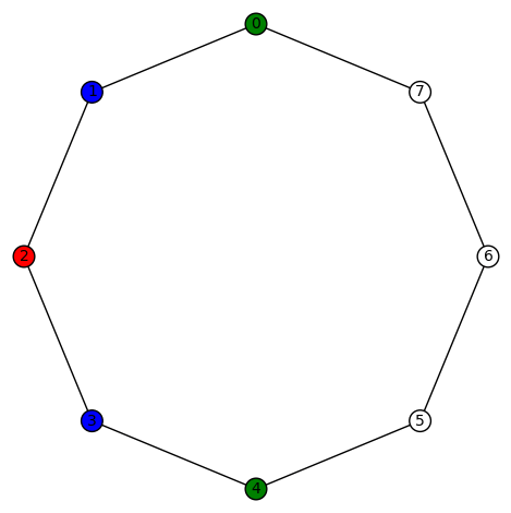
Example 1: There are only the 4 trivial harmonic morphisms $C_6 \to P_4$ , plus that induced by $f = (1, 2, 3, 2, 1, 0)$ and all of its cyclic permutations (4+6=10). This set of 6 permutations is closed under the automorphism of $P_4$ induced by the transposition (0,3)(1,2) (so total = 10). cyclic6-123210

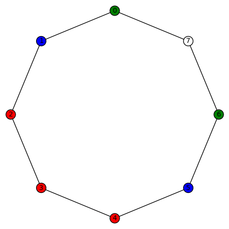
Example 2: There are only the 4 trivial harmonic morphisms, plus $f = (1, 2, 3, 2, 1, 0, 0)$ and all of its cyclic permutations (4+7=11). This set of 7 permutations is not closed under the automorphism of $P_4$ induced by the transposition (0,3)(1,2), so one also has $f = (2, 1, 0, 1, 2, 3, 3)$ and all 7 of its cyclic permutations (total = 7+11 = 18).
cyclic7-1232100
cyclic7-1233210

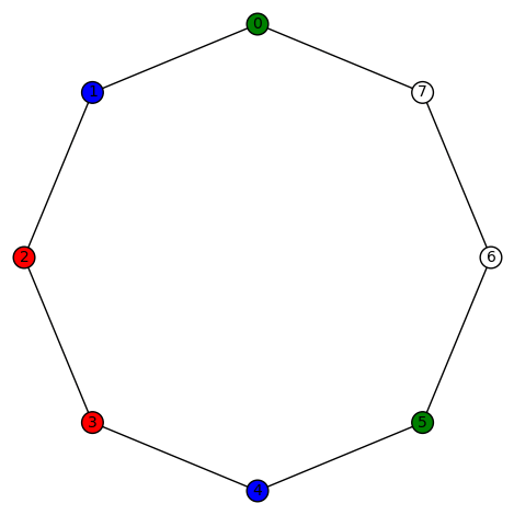
Example 3: There are only the 4 trivial harmonic morphisms, plus $f = (1, 2, 3, 2, 1, 0, 0, 0)$ and all of its cyclic permutations (4+8=12). This set of 8 permutations is not closed under the automorphism of $P_4$ induced by the transposition (0,3)(1,2), so one also has $f = (1, 2, 3, 3, 3, 2, 1, 0)$ and all of its cyclic permutations (12+8=20). In addition, there is $f = (1, 2, 3, 3, 2, 1, 0, 0)$ and all of its cyclic permutations (20+8 = 28). The latter set of 8 cyclic permutations of $(1, 2, 3, 3, 2, 1, 0, 0)$ is closed under the transposition (0,3)(1,2) (total = 28).
cyclic8-12321000
cyclic8-12333210
cyclic8-12332100

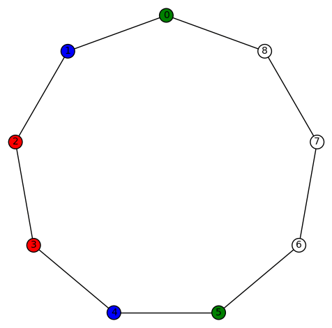
Example 4: There are only the 4 trivial harmonic morphisms, plus $f = (1, 2, 3, 2, 1, 0, 0, 0, 0)$ and all of its cyclic permutations (4+9=13). This set of 9 permutations is not closed under the automorphism of $P_4$ induced by the transposition (0,3)(1,2), so one also has $f = (1, 2, 3, 3, 2, 1, 0, 0, 0)$ and all 9 of its cyclic permutations (9+13 = 22). This set of 9 permutations is not closed under the automorphism of $P_4$ induced by the transposition (0,3)(1,2), so one also has $f = (1, 2, 3, 3, 3, 2, 1, 0, 0)$ and all 9 of its cyclic permutations (9+22 = 31). This set of 9 permutations is not closed under the automorphism of $P_4$ induced by the transposition (0,3)(1,2), so one also has $f = (1, 2, 3, 3, 3, 3, 2, 1, 0)$ and all 9 of its cyclic permutations (total = 9+31 = 40). cyclic9-123210000 cyclic9-123321000 cyclic9-123332100 cyclic9-123333210

Next we consider some cubic graphs.

Example 5: There are 5 cubic graphs on 8 vertices, as listed on this wikipedia page. I wrote a SageMath program that looked for harmonic morphisms on a case-by-case basis. There are no non-trivial harmonic morphisms from any one of these 5 graphs to $P_4$ .

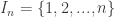
Example 6: There are 19 cubic graphs on 10 vertices, as listed on this wikipedia page. I wrote a SageMath program that looked for harmonic morphisms on a case-by-case basis. The only one of these 19 cubic graphs $\Gamma_1$ having a harmonic morphism $\phi:\Gamma_1\to P_4$ is the graph whose SageMath command is graphs.LCFGraph(10,[5, -3, -3, 3, 3],2). It has diameter 3, girth 4, and automorphism group of order 48 generated by (4,6), (2,8)(3,7), (1,9), (0,2)(3,5), (0,3)(1,4)(2,5)(6,9)(7,8). There are eight non-trivial harmonic morphisms $\phi:\Gamma_1\to P_4$ . They are depicted as follows:
3regular10nn-P4-1112322210
3regular10nn-P4-1112223210
3regular10nn-P4-1012322211
3regular10nn-P4-1012223211
3regular10nn-P4-2321110122
3regular10nn-P4-2321011122
3regular10nn-P4-2221110123
3regular10nn-P4-2221011123
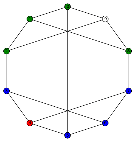
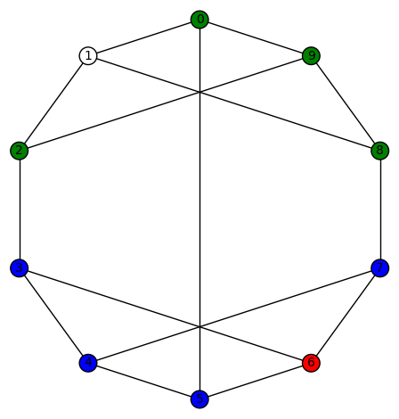
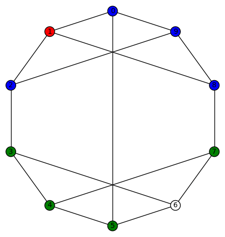
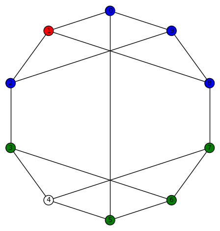
Note that the last four are obtained from the first 4 by applying the permutation (0,3)(1,2) to the colors (where 0 is white, etc, as above).

We move to cubic graphs on 12 vertices. There are quite a few of them – according to the House of Graphs page on connected cubic graphs, there are 109 of them (if I counted correctly).

Example 7: The cubic graphs on 12 vertices are listed on this wikipedia page. I wrote a SageMath program that looked for harmonic morphisms on a case-by-case basis. If there is no harmonic morphism $\Gamma_1\to P_4$ then, instead of showing a graph, I’ll list the edges (of course, the vertices are 0,1,…,11) and the SageMath command for it.

$\Gamma_1=(V_1,E_1)$ , where $E_1=\{ (0, 1), (0, 2), (0, 11), (1, 2), (1, 6), (2, 3), (3, 4), (3, 5), (4, 5), (4, 6), (5, 6), (7, 8), (7, 9), (7, 11), (8, 9), (8, 10), (9, 10), (10, 11)\}$ .
SageMath command:
V1 = [0,1,2,3,4,5,6,7,8,9,10,11] E1 = [(0,1), (0,2), (0,11), (1,2), (1,6),(2,3), (3,4), (3,5), (4,5), (4,6), (5,6), (7,8), (7,9), (7,11), (8,9),(8,10), (9,10), (10,11)] Gamma1 = Graph([V1,E1])
(Not in LCF notation since it doesn’t have a Hamiltonian cycle.)
$\Gamma_1=(V_1,E_1)$ , where $E_1=\{ (0, 1), (0, 6), (0, 11), (1, 2), (1, 3), (2, 3), (2, 5), (3, 4), (4, 5), (4, 6), (5, 6), (7, 8), (7, 9), (7, 11), (8, 9), (8, 10), (9, 10), (10, 11)\}$ .
SageMath command:
V1 = [0,1,2,3,4,5,6,7,8,9,10,11] E1 = [(0, 1), (0, 6), (0, 11), (1, 2), (1, 3), (2, 3), (2, 5), (3, 4), (4, 5), (4, 6), (5, 6), (7, 8), (7, 9), (7, 11), (8, 9), (8, 10), (9, 10), (10, 11)] Gamma1 = Graph([V1,E1])
(Not in LCF notation since it doesn’t have a Hamiltonian cycle.)
$\Gamma_1=(V_1,E_1)$ , where $E_1=\{(0,1),(0,3),(0,11),(1,2),(1,6),(2,3),(2,5),(3,4),(4,5),(4,6),(5,6),(7,8),(7,9),(7,11),(8,9),(8,10),(9,10),(10,11)\}$ .
SageMath command:
V1 = [0,1,2,3,4,5,6,7,8,9,10,11] E1 = [(0,1),(0,3),(0,11),(1,2),(1,6),(2,3),(2,5),(3,4),(4,5),(4,6),(5,6),(7,8),(7,9),(7,11),(8,9),(8,10),(9,10),(10,11)] Gamma1 = Graph([V1,E1])
(Not in LCF notation since it doesn’t have a Hamiltonian cycle.)
$\Gamma_1=(V_1,E_1)$ , where $E_1=\{(0, 1), (0, 3), (0, 11), (1, 2), (1, 11), (2, 3), (2, 10), (3, 4), (4, 5), (4, 8), (5, 6), (5, 7), (6, 7), (6, 9), (7, 8), (8, 9), (9, 10), (10, 11)\}$ .
SageMath command:
Gamma1 = graphs.LCFGraph(12, [3, -2, -4, -3, 4, 2], 2)
$\Gamma_1=(V_1,E_1)$ , where $E_1=\{(0, 1), (0, 3), (0, 11), (1, 2), (1, 11), (2, 3), (2, 10), (3, 4), (4, 5), (4, 7), (5, 6), (5, 8), (6, 7), (6, 9), (7, 8), (8, 9), (9, 10), (10, 11)\}$ .
SageMath command:
Gamma1 = graphs.LCFGraph(12, [3, -2, -4, -3, 3, 3, 3, -3, -3, -3, 4, 2], 1)
$\Gamma_1=(V_1,E_1)$ , where $E_1=\{(0, 1), (0, 4), (0, 11), (1, 2), (1, 3), (2, 3), (2, 5), (3, 4), (4, 5), (5, 6), (6, 7), (6, 8), (7, 8), (7, 10), (8, 9), (9, 10), (9, 11), (10, 11)\}$ .
SageMath command:
Gamma1 = graphs.LCFGraph(12, [4, 2, 3, -2, -4, -3, 2, 3, -2, 2, -3, -2], 1)
$\Gamma_1=(V_1,E_1)$ , where $E_1=\{(0, 1), (0, 3), (0, 11), (1, 2), (1, 4), (2, 3), (2, 5), (3, 4), (4, 5), (5, 6), (6, 7), (6, 9), (7, 8), (7, 10), (8, 9), (8, 11), (9, 10), (10, 11)\}$ .
SageMath command:
Gamma1 = graphs.LCFGraph(12, [3, 3, 3, -3, -3, -3], 2)
(list under construction)