This page is modeled after the handy wikipedia page Table of simple cubic graphs of “small” connected 3-regular graphs, where by small I mean at most 11 vertices.
These graphs are obtained using the SageMath command graphs(n, [4]*n), where n = 5,6,7,… .
5 vertices: Let  denote the vertex set. There is (up to isomorphism) exactly one 4-regular connected graphs on 5 vertices. By Ore’s Theorem, this graph is Hamiltonian. By Euler’s Theorem, it is Eulerian.
4reg5a: The only such 4-regular graph is the complete graph  .
.

We have
- diameter = 1
- girth = 3
- If G denotes the automorphism group then G has cardinality 120 and is generated by (3,4), (2,3), (1,2), (0,1). (In this case, clearly,
 .)
.)
- edge set:

6 vertices: Let 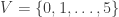 denote the vertex set. There is (up to isomorphism) exactly one 4-regular connected graphs on 6 vertices. By Ore’s Theorem, this graph is Hamiltonian. By Euler’s Theorem, it is Eulerian.
4reg6a: The first (and only) such 4-regular graph is the graph  having edge set:
  .
.

We have
- diameter = 2
- girth = 3
- If G denotes the automorphism group then G has cardinality 48 and is generated by (2,4), (1,2)(4,5), (0,1)(3,5).
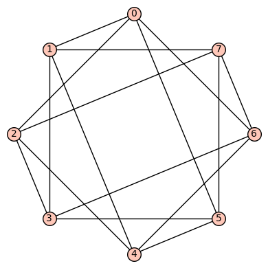
7 vertices: Let  denote the vertex set. There are (up to isomorphism) exactly 2 4-regular connected graphs on 7 vertices. By Ore’s Theorem, these graphs are Hamiltonian. By Euler’s Theorem, they are Eulerian.
4reg7a: The 1st such 4-regular graph is the graph having edge set:  . This is an Eulerian, Hamiltonian (by Ore’s Theorem), vertex transitive (but not edge transitive) graph.

We have
- diameter = 2
- girth = 3
- If G denotes the automorphism group then G has cardinality 14 and is generated by (1,5)(2,4)(3,6), (0,1,3,2,4,6,5).
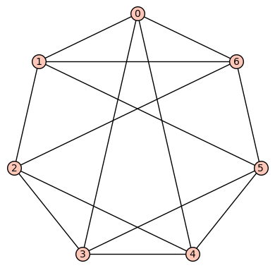
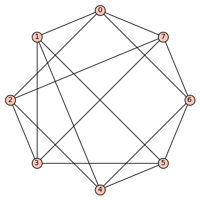
4reg7b: The 2nd such 4-regular graph is the graph having edge set:  . This is an Eulerian, Hamiltonian graph (by Ore’s Theorem) which is neither vertex transitive nor edge transitive.
We have
- diameter = 2
- girth = 3
- If G denotes the automorphism group then G has cardinality 48 and is generated by (3,4), (2,5), (1,3)(4,6), (0,2)
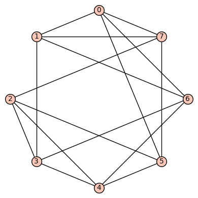
8 vertices: Let  denote the vertex set. There are (up to isomorphism) exactly six 4-regular connected graphs on 8 vertices. By Ore’s Theorem, these graphs are Hamiltonian. By Euler’s Theorem, they are Eulerian.
4reg8a: The 1st such 4-regular graph is the graph having edge set:  . This is vertex transitive but not edge transitive.
We have
- diameter = 2
- girth = 3
- If G denotes the automorphism group then G has cardinality 16 and is generated by
 and
and  .
.
4reg8b: The 2nd such 4-regular graph is the graph having edge set: . This is a vertex transitive (but not edge transitive) graph.
We have
- diameter = 2
- girth = 3
- If G denotes the automorphism group then G has cardinality 48 and is generated by
 ,
,  ,
,  ,
,  .
.
4reg8c: The 3rd such 4-regular graph is the graph having edge set:  . This is a strongly regular (with “trivial” parameters (8, 4, 0, 4)), vertex transitive, edge transitive graph.
We have
- diameter = 2
- girth = 4
- If G denotes the automorphism group then G has cardinality
 and is generated by (5,6), (4,7), (3,4), (2,5), (1,2), (0,1)(2,3)(4,5)(6,7).
4reg8d: The 4th such 4-regular graph is the graph having edge set:  . This graph is not vertex transitive, nor edge transitive.

We have
- diameter = 2
- girth = 3
- If G denotes the automorphism group then G has cardinality 16 and is generated by (3,5), (1,4), (0,2)(1,3)(4,5)(6,7), (0,6)(2,7).
4reg8e: The 5th such 4-regular graph is the graph having edge set:  . This graph is not vertex transitive, nor edge transitive.
We have
- diameter = 2
- girth = 3
- If G denotes the automorphism group then G has cardinality 4 and is generated by (0,1)(2,4)(3,6)(5,7), (0,2)(1,4)(3,6).
4reg8f: The 6th (and last) such 4-regular graph is the bipartite graph  having edge set:
  . This graph is not vertex transitive, nor edge transitive.

We have
- diameter = 2
- girth = 3
- If G denotes the automorphism group then G has cardinality 12 and is generated by (3,4)(6,7), (1,2), (0,3)(5,6).
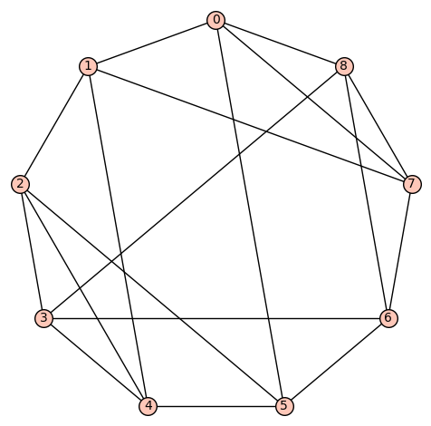
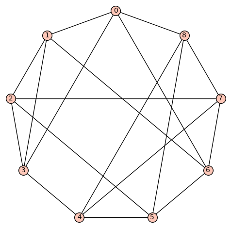
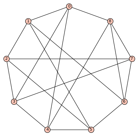
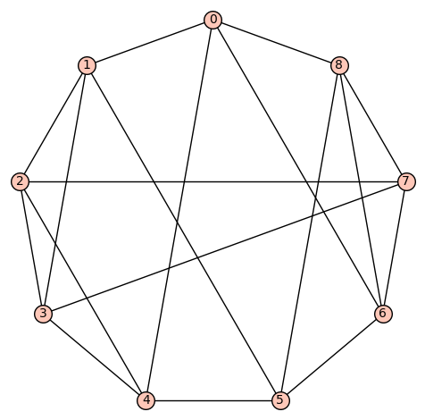
9 vertices: Let  denote the vertex set. There are (up to isomorphism) exactly 16 4-regular connected graphs on 9 vertices. Perhaps the most interesting of these is the strongly regular graph with parameters (9, 4, 1, 2) (also distance regular, as well as vertex- and edge-transitive). It has an automorphism group of cardinality 72, and is referred to as d4reg9-14 below.
Without going into details, it is possible to theoretically prove that there are no harmonic morphisms from any of these graphs to either the cycle graph  or the complete graph
  . However, both d4reg9-3 and d4reg9-14 not only have harmonic morphisms to
  , they each may be regarded as a multicover of .
d4reg9-1
Gamma edges: E1 = [(0, 1), (0, 2), (0, 7), (0, 8), (1, 2), (1, 3), (1, 7), (2, 3), (2, 8), (3, 4), (3, 5), (4, 5), (4, 6), (4, 8), (5, 6), (5, 7), (6, 7), (6, 8)]
diameter:  2
girth:  3
is connected:  True
aut gp size:  12
aut gp gens:  [(1,2)(4,5)(7,8), (0,1)(3,8)(5,6), (0,4)(1,5)(2,6)(3,7)]

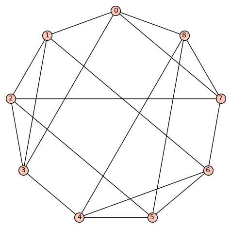
d4reg9-2
Gamma edges: E1 = [(0, 1), (0, 3), (0, 7), (0, 8), (1, 2), (1, 3), (1, 7), (2, 3), (2, 5), (2, 8), (3, 4), (4, 5), (4, 6), (4, 8), (5, 6), (5, 7), (6, 7), (6, 8)]
diameter:  2
girth:  3
is connected:  True
aut gp size:  2
aut gp gens:  [(0,5)(1,6)(2,8)(3,4)]

d4reg9-3
Gamma edges: E1 = [(0, 1), (0, 2), (0, 7), (0, 8), (1, 2), (1, 3), (1, 4), (2, 3), (2, 8), (3, 4), (3, 5), (4, 5), (4, 6), (5, 6), (5, 7), (6, 7), (6, 8), (7, 8)]
diameter:  2
girth:  3
is connected:  True
aut gp size:  18
aut gp gens:  [(1,7)(2,8)(3,6)(4,5), (0,1,4,6,8,2,3,5,7)]

d4reg9-4
Gamma edges: E1 = [(0, 1), (0, 5), (0, 7), (0, 8), (1, 2), (1, 4), (1, 7), (2, 3), (2, 4), (2, 5), (3, 4), (3, 6), (3, 8), (4, 5), (5, 6), (6, 7), (6, 8), (7, 8)]
diameter:  2
girth:  3
is connected:  True
aut gp size:  4
aut gp gens:  [(2,4), (0,6)(1,3)(7,8)]
d4reg9-5
Gamma edges: E1 = [(0, 1), (0, 3), (0, 5), (0, 8), (1, 2), (1, 4), (1, 7), (2, 3), (2, 5), (2, 7), (3, 4), (3, 8), (4, 5), (4, 6), (5, 6), (6, 7), (6, 8), (7, 8)]
diameter:  2
girth:  3
is connected:  True
aut gp size:  12
aut gp gens:  [(1,5)(2,4)(6,7), (0,1)(2,3)(4,5)(7,8)]

d4reg9-6
Gamma edges: E1 = [(0, 1), (0, 3), (0, 7), (0, 8), (1, 2), (1, 5), (1, 6), (2, 3), (2, 5), (2, 6), (3, 4), (3, 8), (4, 5), (4, 7), (4, 8), (5, 6), (6, 7), (7, 8)]
diameter:  2
girth:  3
is connected:  True
aut gp size:  8
aut gp gens:  [(2,6)(3,7), (0,3)(1,2)(4,7)(5,6)]

d4reg9-7
Gamma edges: E1 = [(0, 1), (0, 3), (0, 4), (0, 8), (1, 2), (1, 3), (1, 6), (2, 3), (2, 5), (2, 7), (3, 4), (4, 5), (4, 8), (5, 6), (5, 7), (6, 7), (6, 8), (7, 8)]
diameter:  2
girth:  3
is connected:  True
aut gp size:  2
aut gp gens:  [(0,3)(1,4)(2,8)(5,6)]

d4reg9-8
Gamma edges: E1 = [(0, 1), (0, 3), (0, 7), (0, 8), (1, 2), (1, 3), (1, 6), (2, 3), (2, 5), (2, 7), (3, 4), (4, 5), (4, 6), (4, 8), (5, 6), (5, 8), (6, 7), (7, 8)]
diameter:  2
girth:  3
is connected:  True
aut gp size:  2
aut gp gens:  [(0,8)(1,5)(2,6)(3,4)]
d4reg9-9
Gamma edges: E1 = [(0, 1), (0, 3), (0, 6), (0, 8), (1, 2), (1, 3), (1, 6), (2, 3), (2, 5), (2, 7), (3, 4), (4, 5), (4, 7), (4, 8), (5, 6), (5, 8), (6, 7), (7, 8)]
diameter:  2
girth:  3
is connected:  True
aut gp size:  4
aut gp gens:  [(5,7), (0,3)(2,6)(4,8)]
d4reg9-10
Gamma edges: E1 = [(0, 1), (0, 3), (0, 5), (0, 8), (1, 2), (1, 4), (1, 6), (2, 3), (2, 5), (2, 7), (3, 4), (3, 7), (4, 5), (4, 8), (5, 6), (6, 7), (6, 8), (7, 8)]
diameter:  2
girth:  3
is connected:  True
aut gp size:  16
aut gp gens:  [(2,6)(3,8), (1,5), (0,1)(2,3)(4,5)(6,8)]

d4reg9-11
Gamma edges: E1 = [(0, 1), (0, 3), (0, 7), (0, 8), (1, 2), (1, 4), (1, 6), (2, 3), (2, 5), (2, 7), (3, 4), (3, 5), (4, 5), (4, 8), (5, 6), (6, 7), (6, 8), (7, 8)]
diameter:  2
girth:  3
is connected:  True
aut gp size:  8
aut gp gens:  [(2,4)(7,8), (0,2)(3,7)(4,6)(5,8)]

d4reg9-12
Gamma edges: E1 = [(0, 1), (0, 3), (0, 6), (0, 8), (1, 2), (1, 4), (1, 6), (2, 3), (2, 5), (2, 7), (3, 4), (3, 7), (4, 5), (4, 8), (5, 6), (5, 8), (6, 7), (7, 8)]
diameter:  2
girth:  3
is connected:  True
aut gp size:  18
aut gp gens:  [(1,6)(2,5)(3,8)(4,7), (0,1,6)(2,7,3)(4,5,8), (0,2)(1,3)(5,8(6,7)]

d4reg9-13
Gamma edges: E1 = [(0, 1), (0, 3), (0, 4), (0, 8), (1, 2), (1, 5), (1, 6), (2, 3), (2, 5), (2, 7), (3, 4), (3, 7), (4, 5), (4, 8), (5, 6), (6, 7), (6, 8), (7, 8)]
diameter:  2
girth:  3
is connected:  True
aut gp size:  8
aut gp gens:  [(2,6)(3,8), (0,1)(2,3)(4,5)(6,8), (0,4)(1,5)]
d4reg9-14
Gamma edges: E1 = [(0, 1), (0, 3), (0, 4), (0, 8), (1, 2), (1, 5), (1, 8), (2, 3), (2, 5), (2, 7), (3, 4), (3, 7), (4, 5), (4, 6), (5, 6), (6, 7), (6, 8), (7, 8)]
diameter:  2
girth:  3
is connected:  True
aut gp size:  72
aut gp gens:  [(2,5)(3,4)(6,7), (1,3)(4,8)(5,7), (0,1)(2,3)(4,5)]

d4reg9-15
Gamma edges: E1 = [(0, 1), (0, 4), (0, 6), (0, 8), (1, 2), (1, 3), (1, 5), (2, 3), (2, 4), (2, 7), (3, 4), (3, 7), (4, 5), (5, 6), (5, 8), (6, 7), (6, 8), (7, 8)]
diameter:  2
girth:  3
is connected:  True
aut gp size:  32
aut gp gens:  [(6,8), (2,3), (1,4), (0,1)(2,6)(3,8)(4,5)]
d4reg9-16
Gamma edges: E1 = [(0, 1), (0, 3), (0, 7), (0, 8), (1, 2), (1, 4), (1, 5), (2, 3), (2, 4), (2, 5), (3, 7), (3, 8), (4, 5), (4, 6), (5, 6), (6, 7), (6, 8), (7, 8)]
diameter:  2
girth:  3
is connected:  True
aut gp size:  16
aut gp gens:  [(7,8), (4,5), (0,1)(2,3)(4,7)(5,8), (0,2)(1,3)(4,7)(5,8)]

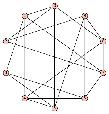
10 vertices: Let  denote the vertex set. There are (up to isomorphism) exactly 59 4-regular connected graphs on 10 vertices. One of these actually has an automorphism group of cardinality 1. According to SageMath: Only three of these are vertex transitive, two (of those 3) are symmetric (i.e., arc transitive), and only one (of those 2) is distance regular.
Example 1: The quartic, symmetric graph on 10 vertices that is not distance regular is depicted below. It has diameter 2, girth 4, chromatic number 3, and has an automorphism group of order 320 generated by  .
.
Example 2: The quartic, distance regular, symmetric graph on 10 vertices is depicted below. It has diameter 3, girth 4, chromatic number 2, and has an automorphism group of order 240 generated by  .
.

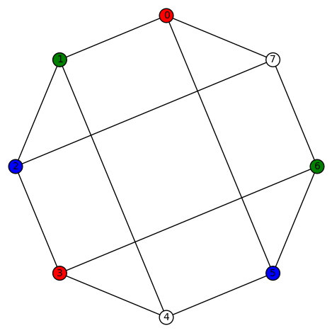
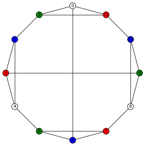
11 vertices: There are (up to isomorphism) exactly 265 4-regular connected graphs on 11 vertices. Only two of these are vertex transitive. None are distance regular or edge transitive.
Example 1: One of the vertex transitive graphs is depicted below. It has diameter 2, girth 4, chromatic number 3, and has an automorphism group of order 22 generated by  .
.
Example 2:The second vertex transitive graph is depicted below. It has diameter 3, girth 3, chromatic number 4, and has an automorphism group of order 22 generated by  .
.
 and
and  . Months of computer searches resulted in a number of conjectures that were used to shape the material in the book.
 be a simple, connected graph with vertices
  and
and  adjacency matrix
  . We start with the geometric series identity
 is the
  denote the orthonormal matrix of normalized eigenvectors, so that
 ,
, 

![\frac{1}{I-tD_\Gamma}= P\cdot [\sum_{\ell=0}^\infty t^\ell A^\ell]\cdot P^{-1}.](https://s0.wp.com/latex.php?latex=%5Cfrac%7B1%7D%7BI-tD_%5CGamma%7D%3D+P%5Ccdot+%5B%5Csum_%7B%5Cell%3D0%7D%5E%5Cinfty+t%5E%5Cell+A%5E%5Cell%5D%5Ccdot+P%5E%7B-1%7D.&bg=ffffff&fg=323232&s=0&c=20201002)

 (i.e.,

 in
in  , we get,
![\sum_{j=0}^{n-1} \lambda_j^{-1}H(f)(\lambda_j^{-1}) = {\frac{1}{\pi}}\sum_{\ell=0}^\infty tr(A^\ell) [M(f)(\ell+1)+(-1)^\ell M(f^*)(\ell+1)],](https://s0.wp.com/latex.php?latex=%5Csum_%7Bj%3D0%7D%5E%7Bn-1%7D+%5Clambda_j%5E%7B-1%7DH%28f%29%28%5Clambda_j%5E%7B-1%7D%29+%3D+%7B%5Cfrac%7B1%7D%7B%5Cpi%7D%7D%5Csum_%7B%5Cell%3D0%7D%5E%5Cinfty+tr%28A%5E%5Cell%29+%5BM%28f%29%28%5Cell%2B1%29%2B%28-1%29%5E%5Cell+M%28f%5E%2A%29%28%5Cell%2B1%29%5D%2C&bg=ffffff&fg=323232&s=0&c=20201002)
 denotes the Hilbert transform
 and
and  is the Mellin transform
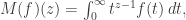
 denotes the negation,
  . Of course, if
  is even then
  , for all
  .
.  can be expressed in terms of the number of walks on the graph: If
  denotes the total number of walks of length
 , where
  is a quotient graph obtained from some subgroup
  . The examples are for graphs having a small number of vertices (no more than 12). For the most part, we also focused on regular graphs with small degree (no more than 5). They were all computed using
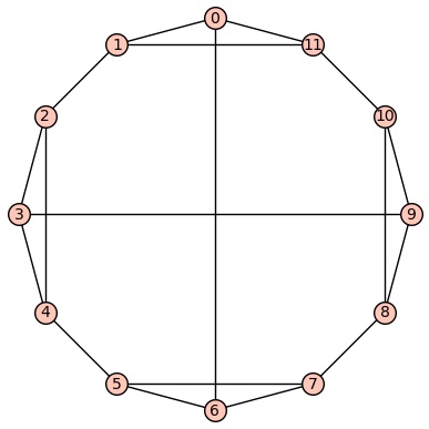

 :
:
 – with no vertical multiplicities and all horizontal multiplicities equal to 1. These 24 harmonic morphisms of
  are all coverings and there are no other harmonic morphisms.
 .
.
 .
.
 to be
to be
 be a harmonic morphism from a graph
  to a graph
  . Then
![{\rm genus}(\Gamma_2)-1 = {\rm deg}(\phi)({\rm genus}(\Gamma_1)-1)+\sum_{x\in V_2} [m_\phi(x)+\frac{1}{2}\nu_\phi(x)-1].](https://s0.wp.com/latex.php?latex=%7B%5Crm+genus%7D%28%5CGamma_2%29-1+%3D+%7B%5Crm+deg%7D%28%5Cphi%29%28%7B%5Crm+genus%7D%28%5CGamma_1%29-1%29%2B%5Csum_%7Bx%5Cin+V_2%7D+%5Bm_%5Cphi%28x%29%2B%5Cfrac%7B1%7D%7B2%7D%5Cnu_%5Cphi%28x%29-1%5D.&bg=ffffff&fg=323232&s=0&c=20201002)
 denotes the horizontal multiplicity and
  denotes the vertical multiplicity.
 -regular and
  -regular.
 be a non-trivial harmonic morphism from a connected


You must be logged in to post a comment.