As in the previous post, let 


The previous post discussed the following result, due to Sturmfels et al.
Theorem: The entry of the matrix A
This post discusses an implementation in Python/Sage.
Consider the following class definition.
class TropicalNumbers:
"""
Implements the tropical semiring.
EXAMPLES:
sage: T = TropicalNumbers()
sage: print T
Tropical Semiring
"""
def __init__(self):
self.identity = Infinity
def __repr__(self):
"""
Called to compute the "official" string representation of an object.
If at all possible, this should look like a valid Python expression
that could be used to recreate an object with the same value.
EXAMPLES:
sage: TropicalNumbers()
TropicalNumbers()
"""
return "TropicalNumbers()"
def __str__(self):
"""
Called to compute the "informal" string description of an object.
EXAMPLES:
sage: T = TropicalNumbers()
sage: print T
Tropical Semiring
"""
return "Tropical Semiring"
def __call__(self, a):
"""
Coerces a into the tropical semiring.
EXAMPLES:
sage: T(10)
TropicalNumber(10)
sage: print T(10)
Tropical element 10 in Tropical Semiring
"""
return TropicalNumber(a)
def __contains__(self, a):
"""
Implements "in".
EXAMPLES:
sage: T = TropicalNumbers()
sage: a = T(10)
sage: a in T
True
"""
if a in RR or a == Infinity:
return a==Infinity or (RR(a) in RR)
else:
return a==Infinity or (RR(a.element) in RR)
class TropicalNumber:
def __init__(self, a):
self.element = a
self.base_ring = TropicalNumbers()
def __repr__(self):
"""
Called to compute the "official" string representation of an object.
If at all possible, this should look like a valid Python expression
that could be used to recreate an object with the same value.
EXAMPLES:
"""
return "TropicalNumber(%s)"%self.element
def __str__(self):
"""
Called to compute the "informal" string description of an object.
EXAMPLES:
sage: T = TropicalNumbers()
sage: print T(10)
Tropical element 10 in Tropical Semiring
"""
return "%s"%(self.number())
def number(self):
return self.element
def __add__(self, other):
"""
Implements +. Assumes both self and other are instances of
TropicalNumber class.
EXAMPLES:
sage: T = TropicalNumbers()
sage: a = T(10)
sage: a in T
True
sage: b = T(15)
sage: a+b
10
"""
T = TropicalNumbers()
return T(min(self.element,other.element))
def __mul__(self, other):
"""
Implements multiplication *.
EXAMPLES:
sage: T = TropicalNumbers()
sage: a = T(10)
sage: a in T
True
sage: b = T(15)
sage: a*b
25
"""
T = TropicalNumbers()
return T(self.element+other.element)
class TropicalMatrix:
def __init__(self, A):
T = TropicalNumbers()
self.base_ring = T
self.row_dimen = len(A)
self.column_dimen = len(A[0])
# now we coerce the entries into T
A0 = A
m = self.row_dimen
n = self.column_dimen
for i in range(m):
for j in range(n):
A0[i][j] = T(A[i][j])
self.array = A0
def matrix(self):
"""
Returns the entries (as ordinary numbers).
EXAMPLES:
sage: A = [[0,1,3,7],[2,0,1,3],[4,5,0,1],[6,3,1,0]]
sage: AT = TropicalMatrix(A)
sage: AT.matrix()
[[0, 1, 3, 7], [2, 0, 1, 3], [4, 5, 0, 1], [6, 3, 1, 0]]
"""
m = self.row_dim()
n = self.column_dim()
A0 = [[0 for i in range(n)] for j in range(m)]
for i in range(m):
for j in range(n):
A0[i][j] = (self.array[i][j]).number()
return A0
def row_dim(self):
return self.row_dimen
def column_dim(self):
return self.column_dimen
def __repr__(self):
"""
Called to compute the "official" string representation of an object.
If at all possible, this should look like a valid Python expression
that could be used to recreate an object with the same value.
EXAMPLES:
"""
return "TropicalMatrix(%s)"%self.array
def __str__(self):
"""
Called to compute the "informal" string description of an object.
EXAMPLES:
"""
return "Tropical matrix %s"%(self.matrix())
def __add__(self, other):
"""
Implements +. Assumes both self and other are instances of
TropicalMatrix class.
EXAMPLES:
sage: A = [[1,2,Infinity],[3,Infinity,0]]
sage: B = [[2,Infinity,1],[3,-1,1]]
sage: AT = TropicalMatrix(A)
sage: BT = TropicalMatrix(B)
sage: AT
TropicalMatrix([[TropicalNumber(1), TropicalNumber(2), TropicalNumber(+Infinity)],
[TropicalNumber(3), TropicalNumber(+Infinity), TropicalNumber(0)]])
sage: AT+BT
[[TropicalNumber(1), TropicalNumber(2), TropicalNumber(1)],
[TropicalNumber(3), TropicalNumber(-1), TropicalNumber(0)]]
"""
A = self.array
B = other.array
C = []
m = self.row_dim()
n = self.column_dim()
if m != other.row_dim:
raise ValueError, "Row dimensions must be equal."
if n != other.column_dim:
raise ValueError, "Column dimensions must be equal."
for i in range(m):
row = [A[i][j]+B[i][j] for j in range(n)] # + as tropical numbers
C.append(row)
return C
def __mul__(self, other):
"""
Implements multiplication *.
EXAMPLES:
sage: A = [[1,2,Infinity],[3,Infinity,0]]
sage: AT = TropicalMatrix(A)
sage: B = [[2,Infinity],[-1,1],[Infinity,0]]
sage: BT = TropicalMatrix(B)
sage: AT*BT
[[TropicalNumber(1), TropicalNumber(3)],
[TropicalNumber(5), TropicalNumber(0)]]
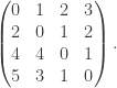
sage: A = [[0,1,3,7],[2,0,1,3],[4,5,0,1],[6,3,1,0]]
sage: AT = TropicalMatrix(A)
sage: A = [[0,1,3,7],[2,0,1,3],[4,5,0,1],[6,3,1,0]]
sage: AT = TropicalMatrix(A)
sage: print AT*AT*AT
Tropical matrix [[0, 1, 2, 3], [2, 0, 1, 2], [4, 4, 0, 1], [5, 3, 1, 0]]
"""
T = TropicalNumbers()
A = self.matrix()
B = other.matrix()
C = []
mA = self.row_dim()
nA = self.column_dim()
mB = other.row_dim()
nB = other.column_dim()
if nA != mB:
raise ValueError, "Column dimension of A and row dimension of B must be equal."
for i in range(mA):
row = []
for j in range(nB):
c = T(Infinity)
for k in range(nA):
c = c+T(A[i][k])*T(B[k][j])
row.append(c.number())
C.append(row)
return TropicalMatrix(C)
This shows that the shortest distances of digraph with adjacency matrix 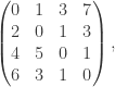
 be a weighted digraph having
  denote its
  adjacency matrix. We identify the vertices with the set
  . In fact, in the latter book, the corresponding section is titled “Dynamic programming”. They formulate it “
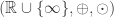 , is defined with the operations as follows:
 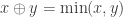 ,
,  . The ordinary product of two
  operations (roughly the same number of additions and multiplications). The tropical product of two
  , where M is the complexity of computing the (tropical) product of two
  time. However, the implied “big-O” constant is so large that the algorithm is not practical. Strassen’s algorithm can multiply two
  time.
time.  , using Strassen’s algorithm. This is better than the
  then this is a
  , which is
  -time algorithm for “dense” graphs. Except for “sparse” graphs, Floyd-Warshall-Roy is better than an interated implementation of Bellman-Ford.
 , for each i, j between 1 and n, then
 (equality is attained, so this is best possible for such matrices).
 is the number of blocks that contain any i-element set of points.
You must be logged in to post a comment.