Review of “Sage: beginner’s guide” by Craig Finch

Posted on 2011/06/11 by wdjoyner

Title: Sage – beginner’s guide

Author: Craig Finch

Technical Reviewers: Dr David Kirkby and Minh Nyugen.

Publisher: Packt Publishing, Open Source series

Review

Complete disclosure: I received this book for free from the publisher, with only the promise to put a review on this blog. Also, I have worked with one of the book’s reviewers (Minh) on a few projects. However, I didn’t receive any other renumeration, don’t know the author of the text under review, and no one asked to pre-approve this review.

The book under review is a book on Sage, an open source mathematical software package started by William Stein, a mathematician at the University of Washington. It is very carefully written (either that, or very carefully reviewed by the Technical Reviewers!) and aimed, as the title suggests, at the beginner. However, it is assumed that the reader knows some undergraduate mathematics, say the level one obtains from getting an engineering degree. In fact, it has a bit of an applied slant with many examples from physics and engineering mathematics. This is a welcome contrast to the excellent Sage Tutorial (available free from the Sage website, http://www.sagemath.org) which has a more of a pure slant. It’s nice to see a publisher like Packt Publishing take the risk of publishing a book like this on an open source software program which already has free documentation (in pdf form).

There are 10 chapters and it’s about 350 pages. Although Sage of course has color plotting, all figures in this book are in black and white, so the reader really must try out the Sage code given in the book to get the full effect. Each chapter features many Time for action Sage code examples (also conveniently listed in the table of contents at the front of the book), followed by a What just happened? section explaining in detail (and without computer code) what the example did. These make the book more useful to the beginner as well as for someone wanting a quick reference for one of the examples. All these examples use the command-line version of Sage (typing your commands into a terminal window at a sage: prompt) but there are several sections explaining the GUI version of Sage (typing your commands into a Mathematica-like “notebook cell”) as well.

Here is a chapter-by-chapter summary:

The first chapter, What can you do with Sage?, is a survey of some of Sage‘s most commonly used capabilities. Examples such as solving a differential equations, plotting experimental data, and some simple example matrix computations are presented.

The second chapter is Installing Sage. This covers the steps you go though for a Mac OS, Windows, and Linux installation of Sage. Since this is scary for a number of users who are not very computer-savvy, it is nice an entire chapter is devoted to this.

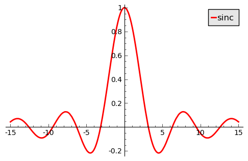
The third chapter, Getting started with Sage, introduces the new Sage user to the user interface, basic Sage syntax, user-defined functions, and some of the available data types (such as strings and real number types). For example, the (black and white version of the) Sage plot of the sinc function,

     sage: f(x) = sin(x)/x
     sage: plot(f, x, xmin=-15, xmax = 15, thickness=2, color="red", legend_label="sinc")

is discussed, among many other things.

This motivates a more detailed introduction to Python, given in the next chapter.

Introducing Python and Sage, the fourth chapter, introduces syntax for Python lists, dictionaries, for loops, if-then statements, and also reading and writing to files. Sage is based on Python, a popular language used extensively in industry (at google among other places). This chapter introduces some very useful stuff, but is pretty basic if you know Python already.

The 5th chapter is Vectors, matrices and linear algebra, and you can guess what it is about. Sage has very wide functionality in linear algebra, with specialized packages for numerical computations for real and complex matrices, matrices over a finite field, or matrices having symbolic coefficients, such as functions of a variable x.

Sage‘s functionality in two-dimensional and three-dimensional plotting is described in the 6th chapter, Plotting with Sage. There is 3-d “live-view” (i.e., you can use the mouse to rotate a plot of a surface or solid in 3-space), histogram plots, as well as simpler plots using Sage‘s 2-d plotting package, matplotlib.

Chapter 7 is Making symbolic mathematics easy. Various topics are covered, from various calculus operations, such as limits, derivatives, integrals, and Laplace transforms, to exact
solutions to equations with variable coefficients, to infinite sums such as power series, to solving ordinary differential equations.

Solving problems numerically is the next chapter. This is the meat-and-potatoes for an applied mathematician. Sage includes many packages which have been developed to solve optimization problems, linear programming problems, numerical solutions of ordinary differential equations, numerical integration, and probability and statistics. These are introduced briefly in this chapter.

The 9th chapter is Learning advanced python programming. Here object-oriented programming is introduced by means of examples, and it is shown how Python handles errors and imports.

The last chapter Where to go from here discusses selected miscellaneous advanced topics.
Topics covered include: LaTeX, interactive plotting using the Sage notebook, as well as a fairly detailed example of analyzing colliding spheres in Sage from several different approaches.

The book has a very good index and, overall I believe is a very welcomed addition to the literature of Sage books.

Zombies and Mathematics

Posted on 2011/05/05 by wdjoyner

What do you do if there is a Zombie attack? Can mathematics help? This post is (humorously) dedicated to collecting links to papers or blog posted related to the mathematical models of Zombies.

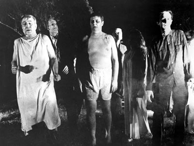
George Romero‘s 1968 Night of the Living Dead, now in the public domain, introduced reanimated ghouls, otherwise known as zombies, which craved live human flesh. Romero’s script was insired on Richard Matheson’s I Am Legend. In Romero’s version, the zombies could be killed by destroying the zombie’s brain. A dead human could, in some cases be “reanimated,” turning into a zombie. These conditions are modeled mathematically in several papers, given below.

When Zombies Attack! Mathematical Modelling of a Zombie Outbreak!, paper by Mathematicians at the University of Ottawa, Philip Munz, Ioan Hudea, Joe Imad and Robert J. Smith? (yes, his last name is spelled “Smith?”).
More Zombie publications by Univ. Ottawa Math Dept Prof. Robert Smith?.
Epidemics in the presence of social attraction and repulsion, Oct 2010 Zombie paper by Evelyn Sander and Chad M. Topaz.
Statistical Inference in a Zombie Outbreak Model, slides for a talk given by Des Higman, May 2010.
Mathematics kills zombies dead!, 08/17/2009 blog post by “Zombie Research Society Staff”.
The Mathematics of Zombies, August 18, 2009 blog post by Mike Elliot.
Love, War and Zombies – Systems of Differential Equations using Sage, April 2011 slides by David Joyner.
This was given on April 22, 2011, as a Project Mosaic/M-cast broadcast.

Public domain 1968 film Night of the Living Dead by George Romero.

Earth Viewed by Apollo 8

Posted on 2011/04/04 by wdjoyner

NASA picture of Planet Earth Earth Viewed by Apollo 8.

God’s number for the Rubik’s cube in the face turn metric

Posted on 2010/08/29 by wdjoyner

This is an update to the older post.

The story is described well at cube20.org but the bottom line is that Tom Rokicki, Herbert Kociemba, Morley Davidson, and John Dethridge have established that every cube position can be solved in 20 face moves or less. The superflip is known to take 20 moves exactly (in 1995, Michael Reid established this), so 20 is best possible – or God’s number in the face turn algorithm. Google (and, earlier, Sony) contributed computer resources to do the needed massive computations. Congradulations to everyone who worked on this!

This would make a great documentary I think!

uniform matroids and MDS codes

Posted on 2010/03/10 by wdjoyner

It is known that uniform (resp. paving) matroids correspond to MDS (resp. “almost MDS” codes). This post explains this connection.

An MDS code is an $[n,k,d]$ linear error correcting block code $C$ which meets the Singleton bound, $d+k=n+1$ . A uniform matroid is a matroid for which all circuits are of size $\geq r(M)+1$ , where $r(M)$ is the rank of M. Recall, a circuit in a matroid M=(E,J) is a minimal dependent subset of E — that is, a dependent set whose proper subsets are all independent (i.e., all in J).

Consider a linear code $C$ whose check matrix is an $(n-k)\times n$ matrix $H=(\vec{h}_1,\dots , \vec{h}_n)$ . The vector matroid M=M[H] is a matroid for which the smallest sized dependency relation among the columns of H is determined by the check relations $c_1\vec{h}_1 + \dots + c_n \vec{h}_n = H\vec{c}=\vec{0}$ , where $\vec{c}=(c_1,\dots,c_n)$ is a codeword (in C which has minimum dimension d). Such a minimum dependency relation of H corresponds to a circuit of M=M[H].

Floyd-Warshall-Roy, 3

Posted on 2010/03/02 by wdjoyner

As in the previous post, let $G=(V,E)$ be a weighted digraph having $n$ vertices and let $A=A_G$ denote its $n\times n$ adjacency matrix. We identify the vertices with the set $\{1,2,\dots, n\}$ .

The previous post discussed the following result, due to Sturmfels et al.

Theorem: The entry of the matrix A^n-1 in row i and column j equals the length of a shortest path from vertex i to vertex j in G. (Here A^n-1 denotes the n-1-st tropical power of A.)

This post discusses an implementation in Python/Sage.

Consider the following class definition.

class TropicalNumbers:
    """
    Implements the tropical semiring.

    EXAMPLES:
        sage: T = TropicalNumbers()
        sage: print T
        Tropical Semiring

    """
    def __init__(self):
        self.identity = Infinity

    def __repr__(self):
        """
        Called to compute the "official" string representation of an object.
        If at all possible, this should look like a valid Python expression
        that could be used to recreate an object with the same value.

        EXAMPLES:
            sage: TropicalNumbers()
            TropicalNumbers()

        """
        return "TropicalNumbers()"

    def __str__(self):
        """
        Called to compute the "informal" string description of an object. 

        EXAMPLES:
            sage: T = TropicalNumbers()
            sage: print T
            Tropical Semiring

        """
        return "Tropical Semiring"

    def __call__(self, a):
        """
        Coerces a into the tropical semiring.

        EXAMPLES:
            sage: T(10)
            TropicalNumber(10)
            sage: print T(10)
            Tropical element 10 in Tropical Semiring
        """
        return TropicalNumber(a)

    def __contains__(self, a):
        """
        Implements "in".

        EXAMPLES:
            sage: T = TropicalNumbers()
            sage: a = T(10)
            sage: a in T
            True

        """
        if a in RR or a == Infinity:
            return a==Infinity or (RR(a) in RR)
        else:
            return a==Infinity or (RR(a.element) in RR)

class TropicalNumber:
    def __init__(self, a):
        self.element = a
        self.base_ring = TropicalNumbers()

    def __repr__(self):
        """
        Called to compute the "official" string representation of an object.
        If at all possible, this should look like a valid Python expression
        that could be used to recreate an object with the same value.

        EXAMPLES:

        """
        return "TropicalNumber(%s)"%self.element

    def __str__(self):
        """
        Called to compute the "informal" string description of an object. 

        EXAMPLES:
            sage: T = TropicalNumbers()
            sage: print T(10)
            Tropical element 10 in Tropical Semiring
        """
        return "%s"%(self.number())

    def number(self):
        return self.element

    def __add__(self, other):
        """
        Implements +. Assumes both self and other are instances of
        TropicalNumber class.

        EXAMPLES:
            sage: T = TropicalNumbers()
            sage: a = T(10)
            sage: a in T
            True
            sage: b = T(15)
            sage: a+b
            10

        """
        T = TropicalNumbers()
        return T(min(self.element,other.element))

    def __mul__(self, other):
        """
        Implements multiplication *.

        EXAMPLES:
            sage: T = TropicalNumbers()
            sage: a = T(10)
            sage: a in T
            True
            sage: b = T(15)
            sage: a*b
            25
        """
        T = TropicalNumbers()
        return T(self.element+other.element)

class TropicalMatrix:
    def __init__(self, A):
        T = TropicalNumbers()
        self.base_ring = T
        self.row_dimen = len(A)
        self.column_dimen = len(A[0])
        # now we coerce the entries into T
        A0 = A
        m = self.row_dimen
        n = self.column_dimen
        for i in range(m):
            for j in range(n):
                A0[i][j] = T(A[i][j])
        self.array = A0

    def matrix(self):
        """
        Returns the entries (as ordinary numbers).

        EXAMPLES:
            sage: A = [[0,1,3,7],[2,0,1,3],[4,5,0,1],[6,3,1,0]]
            sage: AT = TropicalMatrix(A)
            sage: AT.matrix()
            [[0, 1, 3, 7], [2, 0, 1, 3], [4, 5, 0, 1], [6, 3, 1, 0]]
        """
        m = self.row_dim()
        n = self.column_dim()
        A0 = [[0 for i in range(n)] for j in range(m)]
        for i in range(m):
            for j in range(n):
                A0[i][j] = (self.array[i][j]).number()
        return A0

    def row_dim(self):
        return self.row_dimen

    def column_dim(self):
        return self.column_dimen

    def __repr__(self):
        """
        Called to compute the "official" string representation of an object.
        If at all possible, this should look like a valid Python expression
        that could be used to recreate an object with the same value.

        EXAMPLES:

        """
        return "TropicalMatrix(%s)"%self.array

    def __str__(self):
        """
        Called to compute the "informal" string description of an object. 

        EXAMPLES:

        """
        return "Tropical matrix %s"%(self.matrix())

    def __add__(self, other):
        """
        Implements +. Assumes both self and other are instances of
        TropicalMatrix class.

        EXAMPLES:
            sage: A = [[1,2,Infinity],[3,Infinity,0]]
            sage: B = [[2,Infinity,1],[3,-1,1]]
            sage: AT = TropicalMatrix(A)
            sage: BT = TropicalMatrix(B)
            sage: AT
            TropicalMatrix([[TropicalNumber(1), TropicalNumber(2), TropicalNumber(+Infinity)],
              [TropicalNumber(3), TropicalNumber(+Infinity), TropicalNumber(0)]])
            sage: AT+BT
            [[TropicalNumber(1), TropicalNumber(2), TropicalNumber(1)],
             [TropicalNumber(3), TropicalNumber(-1), TropicalNumber(0)]]
        """
        A = self.array
        B = other.array
        C = []
        m = self.row_dim()
        n = self.column_dim()
        if m != other.row_dim:
            raise ValueError, "Row dimensions must be equal."
        if n != other.column_dim:
            raise ValueError, "Column dimensions must be equal."
        for i in range(m):
            row = [A[i][j]+B[i][j] for j in range(n)] # + as tropical numbers
            C.append(row)
        return C

    def __mul__(self, other):
        """
        Implements multiplication *.

        EXAMPLES:
            sage: A = [[1,2,Infinity],[3,Infinity,0]]
            sage: AT = TropicalMatrix(A)
            sage: B = [[2,Infinity],[-1,1],[Infinity,0]]
            sage: BT = TropicalMatrix(B)
            sage: AT*BT
             [[TropicalNumber(1), TropicalNumber(3)],
              [TropicalNumber(5), TropicalNumber(0)]]
            sage: A = [[0,1,3,7],[2,0,1,3],[4,5,0,1],[6,3,1,0]]
            sage: AT = TropicalMatrix(A)
            sage: A = [[0,1,3,7],[2,0,1,3],[4,5,0,1],[6,3,1,0]]
            sage: AT = TropicalMatrix(A)
            sage: print AT*AT*AT
            Tropical matrix [[0, 1, 2, 3], [2, 0, 1, 2], [4, 4, 0, 1], [5, 3, 1, 0]]
        """
        T = TropicalNumbers()
        A = self.matrix()
        B = other.matrix()
        C = []
        mA = self.row_dim()
        nA = self.column_dim()
        mB = other.row_dim()
        nB = other.column_dim()
        if nA != mB:
            raise ValueError, "Column dimension of A and row dimension of B must be equal."
        for i in range(mA):
            row = []
            for j in range(nB):
                c = T(Infinity)
                for k in range(nA):
                    c = c+T(A[i][k])*T(B[k][j])
                row.append(c.number())
            C.append(row)
        return TropicalMatrix(C)

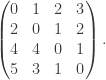
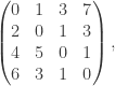
This shows that the shortest distances of digraph with adjacency matrix $\begin{pmatrix} 0&1&3&7\\ 2&0&1&3\\ 4&5&0&1\\ 6&3&1&0\end{pmatrix},$ is equal to A³, which is equal to $\begin{pmatrix} 0&1&2&3\\ 2&0&1&2\\ 4&4&0&1\\ 5&3&1&0\end{pmatrix}.$ This verifies an example given in chapter 1 of the book by Maclagan and Sturmfels, Introduction to Tropical Geometry .

Floyd-Warshall-Roy, 2

Posted on 2010/02/20 by wdjoyner

Let $G = (V,E)$ be a weighted digraph having $n$ vertices and let $A = A_G$ denote its $n \times n$ adjacency matrix. We identify the vertices with the set $\{1,2,\dots, n\}$ . As mentioned in the previous post, the FWR algorithm is an example of dynamic programming. In the book Algebraic Statistics for Computational Biology by L. Pachter and B. Sturmfels, and the book Introduction to Tropical Geometry by D Maclagan and Sturmfels, this algorithm is described using the tropical matrix powers of $A$ . In fact, in the latter book, the corresponding section is titled “Dynamic programming”. They formulate it “tropically” as follows.

Theorem: The entry of the matrix A^n-1 in row i and column j equals the length of a shortest path from vertex i to vertex j in G. (Here A^n-1 denotes the n-1-st tropical power of A.)

How do you compute the tropical power of a matrix? Tropical matrix arithmetic (addition and multiplication) is the obvious extension of the addition and multiplication operations on the tropical semiring. This semiring, $({\mathbb{R}} \cup \{\infty \}, \oplus, \odot)$ , is defined with the operations as follows: $x \oplus y = {\rm min}(x,y)$ , $x \odot y = x+y$ . The ordinary product of two $n\times n$ matrices takes $O(n^3)$ operations (roughly the same number of additions and multiplications). The tropical product of two $n\times n$ matrices still takes $O(n^3)$ operations (but only additions and comparisons, no multiplications). Of course, ordinary powers, as well as tropical powers, can be computed using the repeated squaring algorithm. This implies that the complexity of computing the N-th (tropical) power of an $n \times n$ matrix A is $O(M\log(N))$ , where M is the complexity of computing the (tropical) product of two $n \times n$ matrices.

At the current time, the complexity of ordinary matrix multiplication is best estimated by either Strassen’s algorithm (for practical use) or the Coppersmith-Winograd algorithm (for theoretically best known). The CW algorithm can multiply two $n \times n$ matrices in $O(n^{2.376})$ time. However, the implied “big-O” constant is so large that the algorithm is not practical. Strassen’s algorithm can multiply two $n \times n$ matrices in $O(n^{\log_2(7)+o(1)})=O(n^{2.807})$ time.

Question: Do these complexity estimates extend to tropical matrix multiplication?

If so, then the complexity of computing the matrix A^n-1 is $O(n^{2.807})$ , using Strassen’s algorithm. This is better than the $O(n^3)$ estimate for the FWR algorithm mentioned in the previous post.

In fact, these observations seem so “obvious” that the fact that Sturmfels did not mention them in two different books, makes me wonder if the above question is more difficult to answer than it seems!

Floyd-Warshall-Roy

Posted on 2010/02/08 by wdjoyner

The Floyd-Warshall-Roy algorithm is an algorithm for finding shortest paths in a weighted, directed graph. It allows for negative edge weights and detects a negative weight cycle if one exists. Assuming that there are no negative weight cycles, a single execution of the FWR algorithm will find the shortest paths between all pairs of vertices.

This algorithm is an example of dynamic programming, which allows one to break the computation down to simpler steps using some sort of recursive procedure. If $n=|V|$ then this is a $O(n^3)$ -time algorithm. For comparison, the Bellman-Ford algorithm has complexity $O(|V|\cdot |E|)$ , which is $O(n^3)$ -time for “dense” graphs. However, Bellman-Ford only yields the shortest paths eminating from a single vertex. To achieve comparable output, we would need to iterate Bellman-Ford over all vertices, which would be an $O(n^4)$ -time algorithm for “dense” graphs. Except for “sparse” graphs, Floyd-Warshall-Roy is better than an interated implementation of Bellman-Ford.

Here is a Sage implementation

def floyd_warshall_roy(A):
    """
    Shortest paths

    INPUT: 
        A - weighted adjacency matrix 

    OUTPUT
        dist  - a matrix of distances of shortest paths
        paths - a matrix of shortest paths

    EXAMPLES:
        sage: A = matrix([[0,1,2,3],[0,0,2,1],[20,10,0,3],[11,12,13,0]]); A
        sage: floyd_warshall_roy(A)
        ([[0, 1, 2, 2], [12, 0, 2, 1], [14, 10, 0, 3], [11, 12, 13, 0]], 
          [-1  1  2  1]
          [ 3 -1  2  3]
          [ 3 -1 -1  3]
          [-1 -1 -1 -1])
        sage: A = matrix([[0,1,2,4],[0,0,2,1],[0,0,0,5],[0,0,0,0]])
        sage: floyd_warshall_roy(A)
        ([[0, 1, 2, 2], [+Infinity, 0, 2, 1], [+Infinity, +Infinity, 0, 5],
          [+Infinity, +Infinity, +Infinity, 0]], 
          [-1  1  2  1]
          [-1 -1  2  3]
          [-1 -1 -1  3]
          [-1 -1 -1 -1])
        sage: A = matrix([[0,1,2,3],[0,0,2,1],[-5,0,0,3],[1,0,1,0]]); A
        sage: floyd_warshall_roy(A)
        Traceback (click to the left of this block for traceback)
        ...
        ValueError: A negative edge weight cycle exists.
        sage: A = matrix([[0,1,2,3],[0,0,2,1],[-1/2,0,0,3],[1,0,1,0]]); A
        sage: floyd_warshall_roy(A)
        ([[0, 1, 2, 2], [3/2, 0, 2, 1], [-1/2, 1/2, 0, 3/2], [1/2, 3/2, 1, 0]],
          [-1  1  2  1]
          [ 2 -1  2  3]
          [-1  0 -1  1]
          [ 2  2 -1 -1])
    """
    G = Graph(A, format="weighted_adjacency_matrix")
    V = G.vertices()
    E = [(e[0],e[1]) for e in G.edges()]
    n = len(V)
    dist = [[0]*n for i in range(n)]
    paths = [[-1]*n for i in range(n)]
    # initialization step
    for i in range(n):
        for j in range(n):
            if (i,j) in E:
                paths[i][j] = j
            if i == j:
                dist[i][j] = 0
            elif A[i][j] != 0:
                dist[i][j] = A[i][j]
            else:
                dist[i][j] = infinity
    # iteratively finding the shortest path
    for j in range(n):
        for i in range(n):
            if i != j:
                for k in range(n):
                    if k != j:
                        if dist[i][k]>dist[i][j]+dist[j][k]:
                            paths[i][k] = V[j]
                        dist[i][k] = min(dist[i][k], dist[i][j] +dist[j][k])
    for i in range(n):
        if dist[i][i] < 0:
            raise ValueError, "A negative edge weight cycle exists."
    return dist, matrix(paths)

Sage and the future of mathematics

Posted on 2010/02/04 by wdjoyner

I am not a biologist nor a chemist, and maybe neither are you, but suppose we were. Now, if I described a procedure, in “standard” detail, to produce a result XYZ, you would (based on your reasonably expected expertise in the field), follow the steps you believe were described and either reproduce XYZ or, if I was mistaken, not be able to reproduce XYZ. This is called scientific reproducibility. It is cructial to what I believe is one of the fundamental principles of science, namely Popper’s Falsifiability Criterion.

More and more people are arguing, correctly in my opinion, that in the computational realm, in particular in mathematical research which uses computational experiments, that much higher standards are needed. The Ars Technica article linked above suggests that “it’s time for a major revision of the scientific method.” Also, Victoria Stodden argues one must “facilitate reproducibility. Without this data may be open, but will remain de facto in the ivory tower.” The argument basically is that to reproduce computational mathematical experiments is unreasonably difficult, requiring more that a reasonable expertise. These days, it may in fact (unfortunately) require purchasing very expensive software, or possessing of very sophisticated programming skills, accessibility to special hardware, or (worse) guessing parameters and programming procedures only hinted at by the researcher.

Hopefully, Sage can play the role of a standard bearer for such computational reproducibility. Sage is free, open source and there is a publically available server it runs on (sagenb.org).

What government agencies should require such reproducibility? In my opinion, all scientific funding agencies (NSF, etc) should follow these higher standards of computational accountability.

Bases of representable/vector matroids in Sage

Posted on 2010/02/01 by wdjoyner

A matroid M is specified by a set X of “points” and a collection B of “bases, where $X \subset 2^X$ , satisfying certain conditions (see, for example, Oxley’s book, Matroid theory).

One way to construct a matroid, as it turns out, is to consider a matrix M with coefficients in a field F. The column vectors of M are indexed by the numbers $J = \{1,2,\dots,n\}$ . The collection B of subsets of J associated to the linearly independent column vectors of M of cardinality $r = rank_F(M)$ forms a set of bases of a matroid having points $X=J$ .

How do you compute B? The following Sage code should work.



def independent_sets(mat):
    """
    Finds all independent sets in a vector matroid.

    EXAMPLES:
        sage: M = matrix(GF(2), [[1,0,0,1,1,0],[0,1,0,1,0,1],[0,0,1,0,1,1]])
        sage: M
        [1 0 0 1 1 0]
        [0 1 0 1 0 1]
        [0 0 1 0 1 1]
        sage: independent_sets(M)  
        [[0, 1, 2], [], [0], [1], [0, 1], [2], [0, 2], [1, 2], 
        [0, 1, 4], [4], [0, 4], [1, 4], [0, 1, 5], [5], [0, 5], 
        [1, 5], [0, 2, 3], [3], [0, 3], [2, 3], [0, 2, 5], [2, 5], 
        [0, 3, 4], [3, 4], [0, 3, 5], [3, 5], [0, 4, 5], [4, 5], 
        [1, 2, 3], [1, 3], [1, 2, 4], [2, 4], [1, 3, 4], [1, 3, 5], 
        [1, 4, 5], [2, 3, 4], [2, 3, 5], [2, 4, 5]]
        sage: M = matrix(GF(3), [[1,0,0,1,1,0],[0,1,0,1,0,1],[0,0,1,0,1,1]])
        sage: independent_sets(M)
        [[0, 1, 2], [], [0], [1], [0, 1], [2], [0, 2], [1, 2], 
        [0, 1, 4], [4], [0, 4], [1, 4], [0, 1, 5], [5], [0, 5], 
        [1, 5], [0, 2, 3], [3], [0, 3], [2, 3], [0, 2, 5], [2, 5], 
        [0, 3, 4], [3, 4], [0, 3, 5], [3, 5], [0, 4, 5], [4, 5], 
        [1, 2, 3], [1, 3], [1, 2, 4], [2, 4], [1, 3, 4], [1, 3, 5], 
        [1, 4, 5], [2, 3, 4], [2, 3, 5], [2, 4, 5], [3, 4, 5]]
        sage: M345 = matrix(GF(2), [[1,1,0],[1,0,1],[0,1,1]])
        sage: M345.rank()
        2
        sage: M345 = matrix(GF(3), [[1,1,0],[1,0,1],[0,1,1]])
        sage: M345.rank()
        3
    """
    F = mat.base_ring()
    n = len(mat.columns())
    k = len(mat.rows())
    J = Combinations(n,k)
    indE = []
    for x in J:
        M = matrix([mat.column(x[0]),mat.column(x[1]),mat.column(x[2])])
        if k == M.rank():     # all indep sets of max size
            indE.append(x)
            for y in powerset(x): # all smaller indep sets
                if not(y in indE):
                    indE.append(y)
    return indE

def bases(mat, invariant = False):
    """
    Find all bases in a vector/representable matroid.

    EXAMPLES:
        sage: M = matrix(GF(2), [[1,0,0,1,1,0],[0,1,0,1,0,1],[0,0,1,0,1,1]])
        sage: bases(M)

        [[0, 1, 2],
         [0, 1, 4],
         [0, 1, 5],
         [0, 2, 3],
         [0, 2, 5],
         [0, 3, 4],
         [0, 3, 5],
         [0, 4, 5],
         [1, 2, 3],
         [1, 2, 4],
         [1, 3, 4],
         [1, 3, 5],
         [1, 4, 5],
         [2, 3, 4],
         [2, 3, 5],
         [2, 4, 5]]
        sage: L = [x[1] for x in bases(M, invariant=True)]; L.sort(); L
         [5, 16, 17, 33, 37, 44, 45, 48, 81, 84, 92, 93, 96, 112, 113, 116]
    """
    r = mat.rank()
    ind = independent_sets(mat)
    B = []
    for x in ind:
        if len(x) == r:
            B.append(x)
    B.sort()
    if invariant == True:
        B = [(b,sum([k*2^(k-1) for k in b])) for b in B]
    return B