Remarks on the Hamming [7.4.3] code and Sage

Posted on 2012/02/28 by wdjoyner

This post simply collects some very well-known facts and observations in one place, since I was having a hard time locating a convenient reference.

Let $C$ be the binary Hamming [7,4,3] code defined by the generator matrix $G = \left(\begin{array}{rrrrrrr} 1 & 0 & 0 & 0 & 1 & 1 & 1 \\ 0 & 1 & 0 & 0 & 1 & 1 & 0 \\ 0 & 0 & 1 & 0 & 1 & 0 & 1 \\ 0 & 0 & 0 & 1 & 0 & 1 & 1 \end{array}\right)$ and check matrix $H = \left(\begin{array}{rrrrrrr} 1 & 1 & 1 & 0 & 1 & 0 & 0 \\ 1 & 1 & 0 & 1 & 0 & 1 & 0 \\ 1 & 0 & 1 & 1 & 0 & 0 & 1 \end{array}\right)$ . In other words, this code is the row space of G and the kernel of H. We can enter these into Sage as follows:

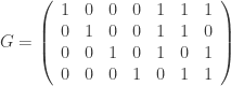
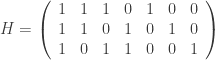
sage: G = matrix(GF(2), [[1,0,0,0,1,1,1],[0,1,0,0,1,1,0],[0,0,1,0,1,0,1],[0,0,0,1,0,1,1]])
sage: G
[1 0 0 0 1 1 1]
[0 1 0 0 1 1 0]
[0 0 1 0 1 0 1]
[0 0 0 1 0 1 1]
sage: H = matrix(GF(2), [[1,1,1,0,1,0,0],[1,1,0,1,0,1,0],[1,0,1,1,0,0,1]])
sage: H
[1 1 1 0 1 0 0]
[1 1 0 1 0 1 0]
[1 0 1 1 0 0 1]
sage: C = LinearCode(G)
sage: C
Linear code of length 7, dimension 4 over Finite Field of size 2
sage: C = LinearCodeFromCheckMatrix(H)
sage: LinearCode(G) == LinearCodeFromCheckMatrix(H)
True

The generator matrix gives us a one-to-one onto map $G:GF(2)^4\to C$ defined by $m \longmapsto m\cdot G$ . Using this map, the codewords are easy to describe and enumerate:

$\begin{tabular}{ccc} decimal & binary & codeword \\ 0 & 0000 & 0000000 \\ 1 & 0001 & 0001011 \\ 2 & 0010 & 0010101 \\ 3 & 0011 & 0011110 \\ 4 & 0100 & 0100110 \\ 5 & 0101 & 0101101 \\ 6 & 0110 & 0110011 \\ 7 & 0111 & 0111000 \\ 8 & 1000 & 1000111 \\ 9 & 1001 & 1001100 \\ 10 & 1010 & 1010010 \\ 11 & 1011 & 1011001 \\ 12 & 1100 & 1100001 \\ 13 & 1101 & 1101010 \\ 14 & 1110 & 1110100 \\ 15 & 1111 & 1111111 \end{tabular}$ .

Using this code, we first describe a guessing game you can play with even small children.

Number Guessing game: Pick an integer from 0 to 15. I will ask you 7 yes/no questions. You may lie once.
I will tell you when you lied and what the correct number is.

Question 1: Is n in {0,1,2,3,4,5,6,7}?
(Translated: Is 1st bit of Hamming_code(n) a 0?)
Question 2: Is n in {0,1,2,3,8,9,10,11}?
(Is 2nd bit of Hamming_code(n) a 0?)
Question 3: Is n in {0,1,4,5,8,9,12,13}?
(Is 3rd bit of Hamming_code(n) a 0?)
Question 4: Is n in {0,2,4,6,8,10,12,14} (ie, is n even)?
(Is 4th bit of Hamming_code(n) a 0?)
Question 5: Is n in {0,1,6,7,10,11,12,13}?
(Is 5th bit of Hamming_code(n) a 0?)
Question 6: Is n in {0,2,5,7,9,11,12,14}?
(Is 6th bit of Hamming_code(n) a 0?)
Question 7: Is n in {0,3,4,7,9,10,13,14}?
(Is 7th bit of Hamming_code(n) a 0?)

Record the answers in a vector (0 for yes, 1 for no): $v = (v_1,v_2,...,v_7)$ . This must be a codeword (no lies) or differ from a codeword by exactly one bit (1 lie). In either case, you can find n by decoding this vector.

We discuss a few decoding algorithms next.

Venn diagram decoding:

We use a simple Venn diagram to describe a decoding method.

sage: t = var('t')
sage: circle1 = parametric_plot([10*cos(t)-5,10*sin(t)+5], (t,0,2*pi))
sage: circle2 = parametric_plot([10*cos(t)+5,10*sin(t)+5], (t,0,2*pi))
sage: circle3 = parametric_plot([10*cos(t),10*sin(t)-5], (t,0,2*pi))
sage: text1 = text("$1$", (0,0))  
sage: text2 = text("$2$", (-6,-2)) 
sage: text3 = text("$3$", (0,7))
sage: text4 = text("$4$", (6,-2)) 
sage: text5 = text("$5$", (-9,9)) 
sage: text6 = text("$6$", (9,9)) 
sage: text7 = text("$7$", (0,-9))  
sage: textA = text("$A$", (-13,13)) 
sage: textB = text("$B$", (13,13)) 
sage: textC = text("$C$", (0,-17)) 
sage: text_all = text1+text2+text3+text4+text5+text6+text7+textA+textB+textC
sage: show(circle1+circle2+circle3+text_all,axes=false)

This gives us the following diagram:

Decoding algorithm:
Suppose you receive $v = ( v_1, v_2, v_3, v_4, v_5, v_6, v_7)$ .
Assume at most one error is made.
Decoding process:

Place $v_i$ in region i of the Venn diagram.
For each of the circles A, B, C, determine if the sum of the bits in four regions add up to 0 or to 1. If they add to 1, say that that circle has a “parity failure”.
The error region is determined form the following table.

$\begin{tabular}{cc} parity failure region(s) & error position \\ none & none \\ A, B, and C & 1 \\ B, C & 4 \\ A, C & 2 \\ A, B & 3 \\ A & 5 \\ B & 6 \\ C & 7 \end{tabular}$

For example, suppose v = (1,1,1,1,1,0,1). The filled in diagram looks like

This only fails in circle B, so the table says (correctly) that the error is in the 6th bit. The decoded codeword is $c = v+e_6 = (1,1,1,1,1,1,1).$

Next, we discuss a decoding method based on the Tanner graph.

Tanner graph for hamming 7,4,3 code

The above Venn diagram corresponds to a bipartite graph, where the left “bit vertices” (1,2,3,4,5,6,7) correspond to the coordinates in the codeword and the right “check vertices” (8,9,10) correspond to the parity check equations as defined by the check matrix. This graph corresponds to the above Venn diagram, where the check vertices 8, 9, 10 were represented by circles A, B, C:

sage: Gamma = Graph({8:[1,2,3,5], 9:[1,2,4,6], 10:[1,3,4,7]})
sage: B = BipartiteGraph(Gamma)
sage: B.show()
sage: B.left
set([1, 2, 3, 4, 5, 6, 7])
sage: B.right
set([8, 9, 10])
sage: B.show()

This gives us the graph in the following picture:

Decoding algorithm:
Suppose you receive $v = ( v_1, v_2, v_3, v_4, v_5, v_6, v_7)$ .
Assume at most one error is made.
Decoding process:

Place $v_i$ at the vertex i on the left side of the bipartite graph.
For each of the check vertices 8,9,10 on the right side of the graph, determine of the if the sum of the bits in the four left-hand vertices connected to it add up to 0 or to 1. If they add to 1, we say that that check vertex has a “parity failure”.
Those check vertices which do not fail are connected to bit vertices which we assume are correct. The remaining bit vertices
connected to check vertices which fail are to be determined (if possible) by solving the corresponding check equations.

check vertex 8: $v_2+v_3+v_4+v_5 = 0$

check vertex 9: $v_1+v_3+v_4+v_6 = 0$

check vertex 10: $v_1+v_2+v_4+v_7 = 0$

Warning: This method is not guaranteed to succeed in general. However, it does work very efficiently when the check matrix H is “sparse” and the number of 1’s in each row and column is “small.”

For example, suppose v = (1,1,1,1,1,0,1). The check vertex 9 fails its parity check, but vertex 8 and 10 do not. Therefore, only bit vertex 6 is unknown, since vertex 6 is the only one not connected to 8 and 10. This tells us that the decoding codeword is $c = (1,1,1,1,1,v_6,1)$ , for some unknown $v_6$ . We solve for this unknown using the check vertex equation $v_1+v_3+v_4+v_6 = 0$ , giving us $v_6 = 1$ . The decoded codeword is $c = (1,1,1,1,1,1,1).$

This last example was pretty simple, so let’s try $v=(0,1,1,1,1,1,1)$ . In this case, we know the vertices 9 and 10 fail, so $c = (v_1,1,1,1,1,v_6,v_7)$ . We solve using

$v_1+1+1+v_6 = 0$

$v_1+1+1+v_7 = 0$

This simply tells us $v_1=v_6=v_7$ . By majority vote, we get $c = (1,1,1,1,1,1,1)$ .

Digital steganography and Sage

Posted on 2012/02/22 by wdjoyner

This post shall explain how the F5 stegosystem (in a simple case) can be implemented in Sage. I thank Carlos Munuera for teaching me these ideas and for many helpful conversations on this matter. I also thank Kyle Tucker-Davis [1] for many interesting conversations on this topic.

Steganography, meaning “covered writing,” is the science of secret communication [4]. The medium used to carry the information is called the “cover” or “stego-cover” (depending on the context – these are not synonymous terms). The term “digital steganography” refers to secret communication where the cover is a digital media file.

One of the most common systems of digital steganography is the Least Significant Bit (LSB) system. In this system, we assume the “cover” image is represented as a finite sequence of binary vectors of a given length. In other words, a greyscale image is regarded as an array of pixels, where each pixel is represented by a binary vector of a certain fixed length. Each such vector represents a pixel’s brightness in the cover image. The encoder embeds (at most) one bit of information in the least significant bit of eaach vector. Care must be taken with this system to ensure that the changes made do not betray the stego-cover, while still maximizing the information hidden.

From a short note of Crandell [3] in 1998, it was realized that error-correcting codes can give rise to “stego-schemes”, ie, methods by which a message can be hidden in a digital file efficiently.

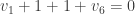
Idea in a nutshell: If $C$ is the r-th binary Hamming code (so, $n = 2^r-1$ is its length, $k = 2^r - r - 1$ is its dimension, and $d = 3$ is its minimum distance), $G$ is a generating matrix, $H$ is a check matrix, and $C^\perp$ is the dual code of $C$ , then we take an element $v \in GF(2)^n$ to be a cover, and the message $m$ we embed is an element of $GF(2)^r$ . 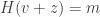Once we find a vector $z$ of lowest weight such that $H(v+z)=m$ , we call $v+z$ the stegocover. The stegocover looks a lot like the original cover and “contains” the message m. This will be explained in more detai below.
(This particular scheme is called the F5 stegosystem, and is due to Westfeld.)

Quick background on error-correcting, linear, block codes [5]

A linear error-correcting block code is a finite dimensional vector space over a finite field with a fixed basis. We assume the finite field is the binary field $GF(2)$ .

We shall typically think of a such a code as a subspace $C$ of $GF(2)^n$ with a fixed basis, where $n>0$ is an integer called the length of the code. Moreover, the basis for the ambient space $GF(2)^n$ will be the standard basis,

$e_1=(1,0,\dots, 0), e_2=(0,1,0,\dots, 0), \dots, e_n=(0,\dots, 0,1).$

There are two common ways to specify a linear code $C$ .

You can give $C$ as a vector subspace of $GF(2)^n$ by specifying a set of basis vectors for $C$ . This set of basis vectors is, by convention, placed as
the rows of a matrix called a generator matrix $G$ of $C$ . Obviously, the order in which the rows are presented does not
affect the code itself.

If $g_1, \dots, g_k$ are the rows of $G$ then

$C= \{c=m_1g_1+\dots +m_kg_k\ |\ {\rm some}\ m_i\in GF(2)\},$

is the set of linear combinations of the row vectors $g_i$ . The vector of coefficients, $m=(m_1,\dots, m_k)$ represents the information you want to encode and transmit.

In other words, encoding of a message can be defined via the generator matrix:

$\begin{array}{ccc} m = (m_1,\dots, m_k) & \to & c=m_1g_1+\dots +m_kg_k = m^t\cdot G,\\ GF(2)^k & \to & C. \end{array}$
You can give $C$ as a vector subspace of $GF(2)^n$ by specifying a matrix $H$ for which $C$ is the kernel of $H$ , $C={\rm ker}(C)$ . This matrix is called a check matrix of $C$ . Again, the order in which the rows are presented does not affect the code itself.

Note that if $G$ is a full rank $k\times n$ matrix then a full rank check matrix $H$ must be a $(n-k) \times n$ matrix.

These two ways of defining a code are not unrelated.

Fact:
If $G=(I_k\ \vert\ A)$ is the generating matrix for $C$ then $H=(-A^t\ \vert\ I_{n-k})$ is a parity check matrix.

Exaample:
Let $r>0$ be an integer and let $H$ be a $r\times (2^r-1)$ matrix whose columns are all the distinct non-zero vectors of $GF(2)^r$ . Then, the code having $H$ as its check matrix is called a binary Hamming code, denoted Ham(r,2).

Let $r=3$ , and let

$H= \begin{pmatrix} 0 & 1 & 1 & 1 & 1 & 0 & 0 \\ 1 & 0 & 1 & 1 & 0 & 1 & 0 \\ 1 & 1 & 0 & 1 & 0 & 0 & 1 \end{pmatrix}.$

In this form, namely when the columns of $H$ are arranged in standard form such that the rightmost $k\times k$ entries is the identity matrix $I_k$ , the generator matrix $G$ can be quickly found to be

$G= \begin{pmatrix} 1 & 0 & 0 & 0 & 0 & 1 & 1 \\ 0 & 1 & 0 & 0 & 1 & 0 & 1 \\ 0 & 0 & 1 & 0 & 1 & 1 & 0 \\ 0 & 0 & 0 & 1 & 1 & 1 & 1 \end{pmatrix}.$

A coset of $GF(2)^n/C$ is a subset of $GF(2)^n$ of the form $C+v$ for some $v\in GF(2)^n$ . Let $S$ be a coset of $C$ . Then,
a coset leader of $S$ is an element of $S$ having smallest Hamming weight.

Fact:
The coset leaders of a Hamming code are those vectors of $wt \leq 1$ .

Steganographic systems from error-correcting codes

This section basically describes Crandell’s idea [3] in a more formalized language.

Following Munuera’s notation in [6], a steganographic system $S$ can be formally defined as

$S= \{\mathcal{C}, \mathcal{M}, \mathcal{K}, emb, rec \},$
where

$\mathcal{C}$ is a set of all possible covers
$\mathcal{M}$ is a set of all possible messages
$\mathcal{K}$ is a set of all possible keys
$emb:\mathcal{C}\times\mathcal{M}\times\mathcal{K}\to\mathcal{C}$ is an embedding function
$rec:\mathcal{C}\times\mathcal{K}\to\mathcal{M}$ is a recovery function

and these all satisfy

$rec(emb(c,m,k),k)=m,$

for all $m\in\mathcal{M}$ , $c\in\mathcal{C}$ , $k\in\mathcal{K}$ . We will assume that a fixed key $k\in\mathcal{K}$ is used, and therefore,
the dependence on an element in the keyspace $\mathcal{K}$ can be ignored. The original cover $c$ is called the plain cover, $m$ is called the message, and $emb(c,m,k)=emb(c,m)$ is called the stegocover. Let $\mathcal{C}$ be $GF(2)^n$ , representing both plain covers and stegocovers. Also, let $\mathcal{M}$ be $GF(2)^k$ , where $k$ is a fixed integer such that $0 \leq k \leq n$ .

Sage examples

How do we compute the emb map?

We need the following Sage function.

def hamming_code_coset_leader(C, y):
      """
      Finds the coset leader of a binary Hamming code C.
      EXAMPLES:
      """
      F = C.base_ring()
      n = C.length()
      k = C.dimension()
      r = n-k
      V0 = F^r
      if not(y in V0):
          RaiseError, "Input vector is not a syndrome."
      H = C.check_mat()
      colsH = H.columns()
      i = colsH.index(y)
      V = F^n
      v = V(0)
      v[i] = F(1)
      return v

Let $V = GF(2)^{63}$ and consider the cover $v = ([1,1,1,1,1,1,1,1,1,1,1,1,1,1,1,1,1,1, 1,1,1,1,0,0,1,1,1, 1,0,0,0,0,0,0,1,1,1,0,0,0,0,0,0,0,1,1,0,0,0,0,0,0,1,1,1,0,0,1,1,0,0,1,1)$ . Regarded as a $7\times 9$ matrix,

V = GF(2)^(63)
rhino = V([1,1,1,1,1,1,1,1,1,
           1,1,1,1,1,1,1,1,1,
           1,1,1,1,0,0,1,1,1,
           1,0,0,0,0,0,0,1,1,
           1,0,0,0,0,0,0,0,1,
           1,0,0,0,0,0,0,1,1,
           1,0,0,1,1,0,0,1,1])
A = matrix(GF(2),7,rhino.list())
matrix_plot(A)

this looks like an elephant or a rhino:

Now we embed the message $m = (1,0,1,0,1,0)$ . First we compute the stegocover:

C = HammingCode(6,GF(2))
H = C.check_mat()
V0 = GF(2)^6
m = V0([1,0,1,0,1,0])
z = hamming_code_coset_leader(C, m)
stegocover = rhino+z
A = matrix(GF(2),7,stegocover.list())
matrix_plot(A)

It looks like another rhino/elephant:

Note only one bit is changed since the Hamming weight of z is at most 1. To recover the message m, just multiply the vector “stegocover” by H.

That’s how you can use Sage to understand the F5 stegosystem, at least in a very simple case.

REFERENCES:
[1] Kyle Tucker-Davis, “An analysis of the F5 steganographic system”, Honors Project 2010-2011
http://www.usna.edu/Users/math/wdj/tucker-davis/

[2] J. Bierbrauer and J. Fridrich. “Constructing good covering codes for applications in Steganography}. 2006.
http://www.math.mtu.edu/jbierbra/.

[3] Crandall, Ron. “Some Notes on Steganography”. Posted on a Steganography Mailing List, 1998.
http://os.inf.tu-dresden.de/westfeld/crandall.pdf

[4] Wayner, Peter. Disappearing Cryptography. Morgan Kauffman Publishers. 2009.

[5] Hill, Raymond. A First Course in Coding Theory. Oxford University Press. 1997.

[6] Munuera, Carlos. “Steganography from a Coding Theory Point of View”. 2010.
http://www.singacom.uva.es/oldsite/Actividad/s3cm/s3cm10/10courses.html

[7] Zhang, Weiming and S. Li. “Steganographic Codes- a New Problem of Coding Theory”. preprint, 2005.
http://arxiv.org/abs/cs/0505072.

Applications of graphs to Boolean functions

Posted on 2012/02/16 by wdjoyner

Let f be a Boolean function on $GF(2)^n$ . The Cayley graph of f is defined to be the graph

$\Gamma_f = (GF(2)^n, E_f )$ ,

whose vertex set is $GF(2)^n$ and the set of edges is defined by

$E_f =\{ (u,v) \in GF(2)^n \times GF(2)^n \ |\ f(u+v)=1\}$ .

The adjacency matrix $A_f$ is the matrix whose entries are

$A_{i,j} = f(b(i) + b(j))$ ,

where b(k) is the binary representation of the integer k.
Note $\Gamma_f$ is a regular graph of degree wt(f), where wt denotes the Hamming weight of f when regarded as a vector of values (of length $2^n$ ).

Recall that, given a graph $\Gamma$ and its adjacency matrix A, the spectrum Spec( $\Gamma$ ) is the multi-set of eigenvalues of A.

The Walsh transform of a Boolean function f is an integer-valued function over $GF(2)^n$ that can be defined as

$W_f(u) = \sum_{x in GF(2)^n} (-1)^{f(x)+ \langle u,x\rangle}.$
A Boolean function f is bent if $|W_f(a)| = 2^{n/2}$ (this only makes sense if n is even). The Hadamard transform of a integer-valued function f is an integer-valued function over $GF(2)^n$ that can be defined as

$H_f(u) = \sum_{x in GF(2)^n} f(x)(-1)^{\langle u,x\rangle}.$
It turns out that the spectrum of $\Gamma_f$ is equal to the Hadamard transform of f when regarded as a vector of (integer) 0,1-values. (This nice fact seems to have first appeared in [2], [3].)

A graph is regular of degree r (or r-regular) if every vertex has degree r (number of edges incident to it).   We say that an r-regular graph $\Gamma$ is a strongly regular graph with parameters (v, r, d, e) (for nonnegative integers e, d) provided, for all vertices u, v the number of vertices adjacent to both u, v is equal to

          e, if u, v are adjacent,
          d, if u, v are nonadjacent.

It turns out tht f is bent iff $\Gamma_f$ is strongly regular and e = d (see [3] and [4]).

The following Sage computations illustrate these and other theorems in [1], [2], [3], [4].

Consider the Boolean function $f: GF(2)^4 \to GF(2)$ given by $f(x_0,x_1,x_2) = x_0x_1+x_2x_3$ .

sage: V = GF(2)^4
sage: f = lambda x: x[0]*x[1]+x[2]*x[3]
sage: CartesianProduct(range(16), range(16))
Cartesian product of [0, 1, 2, 3, 4, 5, 6, 7, 8, 9, 10, 11, 12, 13, 14, 15], 
                     [0, 1, 2, 3, 4, 5, 6, 7, 8, 9, 10, 11, 12, 13, 14, 15]
sage: C = CartesianProduct(range(16), range(16))
sage: Vlist = V.list()                  
sage: E = [(x[0],x[1]) for x in C if f(Vlist[x[0]]+Vlist[x[1]])==1]
sage: len(E)
96
sage: E = Set([Set(s) for s in E])
sage: E = [tuple(s) for s in E] 
sage: Gamma = Graph(E)
sage: Gamma
Graph on 16 vertices
sage: VG = Gamma.vertices()
sage: L1 = []
sage: L2 = []
sage: for v1 in VG:
....:         for v2 in VG:
....:             N1 = Gamma.neighbors(v1)
....:         N2 = Gamma.neighbors(v2)
....:         if v1 in N2:
....:                 L1 = L1+[len([x for x in N1 if x in N2])]
....:         if not(v1 in N2) and v1!=v2:
....:                 L2 = L2+[len([x for x in N1 if x in N2])]
....: 
....: 
sage: L1; L2
[2, 2, 2, 2, 2, 2, 2, 2, 2, 2, 2, 2, 2, 2, 2, 2, 2, 2, 2, 2,
 2, 2, 2, 2, 2, 2, 2, 2, 2, 2, 2, 2, 2, 2, 2, 2, 2, 2, 2, 2,
 2, 2, 2, 2, 2, 2, 2, 2, 2, 2, 2, 2, 2, 2, 2, 2, 2, 2, 2, 2,
 2, 2, 2, 2, 2, 2, 2, 2, 2, 2, 2, 2, 2, 2, 2, 2, 2, 2, 2, 2,
 2, 2, 2, 2, 2, 2, 2, 2, 2, 2, 2, 2, 2, 2, 2, 2]
[2, 2, 2, 2, 2, 2, 2, 2, 2, 2, 2, 2, 2, 2, 2, 2, 2, 2, 2, 2,
 2, 2, 2, 2, 2, 2, 2, 2, 2, 2, 2, 2, 2, 2, 2, 2, 2, 2, 2, 2,
 2, 2, 2, 2, 2, 2, 2, 2, 2, 2, 2, 2, 2, 2, 2, 2, 2, 2, 2, 2,
 2, 2, 2, 2, 2, 2, 2, 2, 2, 2, 2, 2, 2, 2, 2, 2, 2, 2, 2, 2,
 2, 2, 2, 2, 2, 2, 2, 2, 2, 2, 2, 2, 2, 2, 2, 2, 2, 2, 2, 2,
 2, 2, 2, 2, 2, 2, 2, 2, 2, 2, 2, 2, 2, 2, 2, 2, 2, 2, 2, 2,
 2, 2, 2, 2, 2, 2, 2, 2, 2, 2, 2, 2, 2, 2, 2, 2, 2, 2, 2, 2,
 2, 2, 2, 2]

This implies the graph is strongly regular with d=e=2.

sage: Gamma.spectrum()
[6, 2, 2, 2, 2, 2, 2, -2, -2, -2, -2, -2, -2, -2, -2, -2]
sage: [walsh_transform(f, a) for a in V]
[4, 4, 4, -4, 4, 4, 4, -4, 4, 4, 4, -4, -4, -4, -4, 4]
sage: Omega_f = [v for v in V if f(v)==1] 
sage: len(Omega_f)
6
sage: Gamma.is_bipartite()
False
sage: Gamma.is_hamiltonian()
True
sage: Gamma.is_planar()     
False
sage: Gamma.is_regular()
True
sage: Gamma.is_eulerian()
True
sage: Gamma.is_connected()
True
sage: Gamma.is_triangle_free()
False
sage: Gamma.diameter()
2
sage: Gamma.degree_sequence()
[6, 6, 6, 6, 6, 6, 6, 6, 6, 6, 6, 6, 6, 6, 6, 6]
sage: show(Gamma)
# bent-fcns-cayley-graphs1.png

Here is the picture of the graph:

sage: H = matrix(QQ, 16, 16, [(-1)^(Vlist[x[0]]).dot_product(Vlist[x[1]]) for x in C])
sage: H
[ 1  1  1  1  1  1  1  1  1  1  1  1  1  1  1  1]
[ 1 -1  1 -1  1 -1  1 -1  1 -1  1 -1  1 -1  1 -1]
[ 1  1 -1 -1  1  1 -1 -1  1  1 -1 -1  1  1 -1 -1]
[ 1 -1 -1  1  1 -1 -1  1  1 -1 -1  1  1 -1 -1  1]
[ 1  1  1  1 -1 -1 -1 -1  1  1  1  1 -1 -1 -1 -1]
[ 1 -1  1 -1 -1  1 -1  1  1 -1  1 -1 -1  1 -1  1]
[ 1  1 -1 -1 -1 -1  1  1  1  1 -1 -1 -1 -1  1  1]
[ 1 -1 -1  1 -1  1  1 -1  1 -1 -1  1 -1  1  1 -1]
[ 1  1  1  1  1  1  1  1 -1 -1 -1 -1 -1 -1 -1 -1]
[ 1 -1  1 -1  1 -1  1 -1 -1  1 -1  1 -1  1 -1  1]
[ 1  1 -1 -1  1  1 -1 -1 -1 -1  1  1 -1 -1  1  1]
[ 1 -1 -1  1  1 -1 -1  1 -1  1  1 -1 -1  1  1 -1]
[ 1  1  1  1 -1 -1 -1 -1 -1 -1 -1 -1  1  1  1  1]
[ 1 -1  1 -1 -1  1 -1  1 -1  1 -1  1  1 -1  1 -1]
[ 1  1 -1 -1 -1 -1  1  1 -1 -1  1  1  1  1 -1 -1]
[ 1 -1 -1  1 -1  1  1 -1 -1  1  1 -1  1 -1 -1  1]
sage: flist = vector(QQ, [int(f(v)) for v in V])
sage: H*flist  
(6, -2, -2, 2, -2, -2, -2, 2, -2, -2, -2, 2, 2, 2, 2, -2)
sage: A = matrix(QQ, 16, 16, [f(Vlist[x[0]]+Vlist[x[1]]) for x in C])
sage: A.eigenvalues()
[6, 2, 2, 2, 2, 2, 2, -2, -2, -2, -2, -2, -2, -2, -2, -2]

Here is another example: $f: GF(2)^3 \to GF(2)$ given by $f(x_0,x_1,x_2) = x_0x_1+x_2$ .

sage: V = GF(2)^3
sage: f = lambda x: x[0]*x[1]+x[2]
sage: Omega_f = [v for v in V if f(v)==1] 
sage: len(Omega_f)
4
sage: C = CartesianProduct(range(8), range(8))
sage: Vlist = V.list()    
sage: E = [(x[0],x[1]) for x in C if f(Vlist[x[0]]+Vlist[x[1]])==1]
sage: E = Set([Set(s) for s in E])
sage: E = [tuple(s) for s in E] 
sage: Gamma = Graph(E)
sage: Gamma
Graph on 8 vertices
sage: 
sage: VG = Gamma.vertices()
sage: L1 = []
sage: L2 = []
sage: for v1 in VG:
....:         for v2 in VG:
....:             N1 = Gamma.neighbors(v1)
....:         N2 = Gamma.neighbors(v2)
....:         if v1 in N2:
....:                 L1 = L1+[len([x for x in N1 if x in N2])]
....:         if not(v1 in N2) and v1!=v2:
....:                 L2 = L2+[len([x for x in N1 if x in N2])]
....: 
sage: L1; L2
[2, 0, 2, 2, 2, 2, 0, 2, 2, 2, 0, 2, 2, 2, 2, 0, 0, 2, 2, 2, 2, 0, 2, 2, 2, 0, 2, 2, 2, 2, 0, 2]
[2, 2, 2, 2, 2, 2, 2, 2, 2, 2, 2, 2, 2, 2, 2, 2, 2, 2, 2, 2, 2, 2, 2, 2]

This implies that the graph is not strongly regular, therefore f is not bent.

sage: Gamma.spectrum()
[4, 2, 0, 0, 0, -2, -2, -2]
sage: 
sage: Gamma.is_bipartite()
False
sage: Gamma.is_hamiltonian()
True
sage: Gamma.is_planar()     
False
sage: Gamma.is_regular()
True
sage: Gamma.is_eulerian()
True
sage: Gamma.is_connected()
True
sage: Gamma.is_triangle_free()
False
sage: Gamma.diameter()
2
sage: Gamma.degree_sequence()
[4, 4, 4, 4, 4, 4, 4, 4]
sage: H = matrix(QQ, 8, 8, [(-1)^(Vlist[x[0]]).dot_product(Vlist[x[1]]) for x in C])
sage: H
[ 1  1  1  1  1  1  1  1]
[ 1 -1  1 -1  1 -1  1 -1]
[ 1  1 -1 -1  1  1 -1 -1]
[ 1 -1 -1  1  1 -1 -1  1]
[ 1  1  1  1 -1 -1 -1 -1]
[ 1 -1  1 -1 -1  1 -1  1]
[ 1  1 -1 -1 -1 -1  1  1]
[ 1 -1 -1  1 -1  1  1 -1]
sage: flist = vector(QQ, [int(f(v)) for v in V])
sage: H*flist  
(4, 0, 0, 0, -2, -2, -2, 2)
sage: Gamma.spectrum()
[4, 2, 0, 0, 0, -2, -2, -2]
sage: A = matrix(QQ, 8, 8, [f(Vlist[x[0]]+Vlist[x[1]]) for x in C])
sage: A.eigenvalues()
[4, 2, 0, 0, 0, -2, -2, -2]

sage: show(Gamma)
# bent-fcns-cayley-graphs2.png

Here is the picture:

REFERENCES:
[1] Pantelimon Stanica, Graph eigenvalues and Walsh spectrum of Boolean functions, INTEGERS 7(2) (2007), #A32.

[2] Anna Bernasconi, Mathematical techniques for the analysis of Boolean functions, Ph. D. dissertation TD-2/98, Universit di Pisa-Udine, 1998.

[3] Anna Bernasconi and Bruno Codenotti, Spectral Analysis of Boolean Functions as a Graph Eigenvalue Problem, IEEE TRANSACTIONS ON COMPUTERS, VOL. 48, NO. 3, MARCH 1999.

[4] A. Bernasconi, B. Codenotti, J.M. VanderKam. A Characterization of Bent Functions in terms of Strongly Regular Graphs, IEEE Transactions on Computers, 50:9 (2001), 984-985.

[5] Michel Mitton, Minimal polynomial of Cayley graph adjacency matrix for Boolean functions, preprint, 2007.

[6] ——, On the Walsh-Fourier analysis of Boolean functions, preprint, 2006.

Yet Another Mathblog

Monthly Archives: February 2012

Remarks on the Hamming [7.4.3] code and Sage

Digital steganography and Sage

Applications of graphs to Boolean functions