This is the third of a series of expository posts on matrix-theoretic sports ranking methods. This post discusses the random walker ranking.

We follow the presentation in the paper by Govan and Meyer (Ranking National Football League teams using Google’s PageRank). The table of “score differentials” based on the table in a previous post is:

This leads to the following matrix:

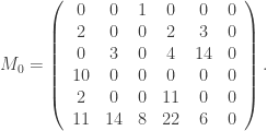
The edge-weighted score-differential graph associated to (regarded as a weighted adjacency matrix) is in the figure below.

This matrix must be normalized to create a (row) stochastic matrix:

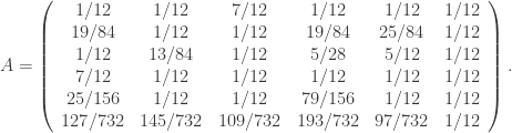
Next, to insure it is irreducible, we replace by , where is the doubly stochastic matrix with every entry equal to :

Let

The ranking determined by the random walker method is the reverse of the left eigenvector of associated to the largest eigenvalue (by reverse, I mean that the vector ranks the teams from worst-to-best, not from best-to-worst, as we have seen in previous ranking methods).
In other words, the vector

This is approximately

Its reverse gives the ranking:

Army Lafayette Bucknell Lehigh Holy Cross Navy.

This gives a prediction failure rate of .