Sports ranking methods, 2

Posted on 2016/12/18 by wdjoyner

This is the second of a series of expository posts on matrix-theoretic sports ranking methods. This post discusses Keener’s method (see J.P. Keener, The Perron-Frobenius theorem and the ranking of football, SIAM Review 35 (1993)80-93 for details).

See the first post in the series for a discussion of the data we’re using to explain this method. We recall the table of results:

X\Y	Army	Bucknell	Holy Cross	Lafayette	Lehigh	Navy
Army	x	14-16	14-13	14-24	10-12	8-19
Bucknell	16-14	x	27-30	18-16	23-20	10-22
Holy Cross	13-14	30-27	x	19-15	17-13	9-16
Lafayette	24-14	16-18	15-19	x	12-23	17-39
Lehigh	12-10	20-23	13-17	23-12	x	12-18
Navy	19-8	22-10	16-9	39-17	18-12	x

sm261_baseball-ranking-application_teams-digraph

Win-loss digraph of the Patriot league mens baseball from 2015

Suppose T teams play each other. Let $A=(a_{ij})_{1\leq i,j\leq T}$ be a non-negative square matrix determined by the results of their games, called the preference matrix. In his 1993 paper, Keener defined the score of the $i$ th team to be given by

$s_i = \frac{1}{n_i}\sum_{j=1}^T a_{ij}r_j,$

where $n_i$ denotes the total number of games played by team $i$ and ${\bf r}=(r_1,r_2,\dots ,r_T)$ is the rating vector (where $r_i\geq 0$ denotes the rating of team $i$ ).

One possible preference matrix the matrix $A$ of total scores obtained from the pre-tournament table below:

$A = \left(\begin{array}{rrrrrr} 0 & 14 & 14 & 14 & 10 & 8 \\ 16 & 0 & 27 & 18 & 23 & 28 \\ 13 & 30 & 0 & 19 & 27 & 43 \\ 24 & 16 & 15 & 0 & 12 & 17 \\ 12 & 20 & 43 & 23 & 0 & 12 \\ 19 & 42 & 30 & 39 & 18 & 0 \end{array}\right),$

(In this case, $n_i=4$ so we ignore the $1/n_i$ factor.)

In his paper, Keener proposed a ranking method where the ranking vector ${\bf r}$ is proportional to its score. The score is expressed as a matrix product $A{\bf r}$ , where $A$ is a square preference matrix. In other words, there is a constant $\rho>0$ such that $s_i=\rho r_i$ , for each $i$ . This is the same as saying $A {\bf r} = \rho {\bf r}$ .

The Frobenius-Perron theorem implies that $S$ has an eigenvector ${\bf r}=(r_1,r_2,r_3,r_4,r_5,r_6)$ having positive entries associated to the largest eigenvalue $\lambda_{max}$ of $A$ , which has (geometric) multiplicity $1$ . Indeed, $A$ has maximum eigenvalue $\lambda_{max}= 110.0385...$ , of multiplicity $1$ , with eigenvector

${\bf r}=(1, 1.8313\dots , 2.1548\dots , 1.3177\dots , 1.8015\dots , 2.2208\dots ).$

Therefore the teams, according to Kenner’s method, are ranked,

Army $<$ Lafayette $<$ Lehigh $<$ Bucknell $<$ Holy Cross $<$ Navy.

This gives a prediction failure rate of just $6.7\%$ .

Memories of TS Michael, by Thomas Quint

Posted on 2016/12/08 by wdjoyner

TS Michael passed away on November 22, 2016, from cancer. I will miss him as a colleague and a kind, wise soul. Tom Quint has kindly allowed me to post these reminiscences that he wrote up.

Well, I guess I could start with the reason TS and I met in the first place. I was a postdoc at USNA in about 1991 and pretty impressed with myself. So when USNA offered to continue my postdoc for two more years (rather than give me a tenure track position), I turned it down. Smartest move I ever made, because TS got the position and so we got to know each other.

We started working w each other one day when we both attended a talk on “sphere of influence graphs”. I found the subject moderately interesting, but he came into my office all excited, and I couldn’t get rid of him — wouldn’t leave until we had developed a few research ideas.

Interestingly, his position at USNA turned into a tenure track, while mine didn’t. It wasn’t until 1996 that I got my position at U of Nevada.

Work sessions with him always followed the same pattern. As you may or may not know, T.S. a) refused to fly in airplanes, and b) didn’t drive. Living across the country from each other, the only way we could work together face-to-face was: once each summer I would fly out to the east coast to visit my parents, borrow one of their cars for a week, and drive down to Annapolis. First thing we’d do is go to Whole Foods, where he would load up my car with food and other supplies, enough to last at least a few months. My reward was that he always bought me the biggest package of nigiri sushi we could find — not cheap at Whole Foods!

It was fun, even though I had to suffer through eight million stories about the USNA Water Polo Team.

Oh yes, and he used to encourage me to sneak into one of the USNA gyms to work out. We figured that no one would notice if I wore my Nevada sweats (our color is also dark blue, and the pants also had a big “N” on them). It worked.

Truth be told, TS didn’t really have a family of his own, so I think he considered the mids as his family. He cared deeply about them (with bonus points if you were a math major or a water polo player :-).

One more TS anecdote, complete with photo. Specifically, TS was especially thrilled to find out that we had named our firstborn son Theodore Saul Quint. Naturally, TS took to calling him “Little TS”. At any rate, the photo below is of “Big TS” holding “Little TS”, some time in the Fall of 2000.

TS Michael in 2000.

Simple unsolved math problem, 7

Posted on 2016/12/07 by wdjoyner

Everyone’s heard of the number $\pi =$ 3.141592…, right?

Robert Couse-Baker / CC BY http://2.0 / Flickr: 29233640@N07

And you probably know that $\pi$ is not a rational number (i.e., a quotient of two integers, like 7/3). Unlike a rational number, whose decimal expansion is eventually periodic, if you look at the digits of $\pi$ they seem random,

3.1415926535897932384626433832795028841971693993751058209749445923078164062862089986280348253421170679821480865132823066470938446095505822317253594081284811174502841027019385211055596446229489549303819644288109756659334461284756482…

But are they really? No one really knows. There’s a paper that explores the statistics of these digits using the first 22.4 trillion digits of $\pi$ . Does any finite sequence of k digits (say, for example, the 4-digit sequence 2016) occur just as often as any other sequence of the same length (say, 1492), for each k? When the answer is yes, the number is called ‘normal.’ That is, a normal number is a real number whose infinite sequence of digits is distributed uniformly in the sense that each digit has the same natural density 1/10, also all possible k-tuples of digits are equally likely with density 1/k, for any integer $k>1$ .

The following simple problem is unsolved:

Conjecture: $\pi$ is normal.

Sports ranking methods, 1

Posted on 2016/12/03 by wdjoyner

This is the first of a series of expository posts on matrix-theoretic sports ranking methods. This post, which owes much to discussions with TS Michael, discusses Massey’s method.

Massey’s method, currently in use by the NCAA (for football, where teams typically play each other once), was developed by Kenneth P. Massey
while an undergraduate math major in the late 1990s. We present a possible variation of Massey’s method adapted to baseball, where teams typically play each other multiple times.

There are exactly 15 pairing between these teams. These pairs are sorted lexicographically, as follows:

(1,2),(1,3),(1,4), …, (5,6).

In other words, sorted as

Army vs Bucknell, Army vs Holy Cross, Army vs Lafayette, …, Lehigh vs Navy.

The cumulative results of the 2016 regular season are given in the table below. We count only the games played in the Patriot league, but not including the Patriot league post-season tournament (see eg, the Patriot League site for details). In the table, the total score (since the teams play multiple games against each other) of the team in the vertical column on the left is listed first. In other words, ”a – b” in row $i$ and column $j$ means the total runs scored by team $i$ against team $j$ is $a$ , and the total runs allowed by team $i$ against team $j$ is $b$ . Here, we order the six teams as above (team $1$ is Army (USMI at Westpoint), team $2$ is Bucknell, and so on). For instance if X played Y and the scores were $10-0$ , $0-1$ , $0-1$ , $0-1$ , $0-1$ , $0-1$ , then the table would read $10-5$ in the position of row X and column Y.

X\Y	Army	Bucknell	Holy Cross	Lafayette	Lehigh	Navy
Army	x	14-16	14-13	14-24	10-12	8-19
Bucknell	16-14	x	27-30	18-16	23-20	10-22
Holy Cross	13-14	30-27	x	19-15	17-13	9-16
Lafayette	24-14	16-18	15-19	x	12-23	17-39
Lehigh	12-10	20-23	13-17	23-12	x	12-18
Navy	19-8	22-10	16-9	39-17	18-12	x

Win-loss digraph of the Patriot league mens baseball from 2015

In this ordering, we record their (sum total) win-loss record (a 1 for a win, -1 for a loss) in a $15\times 6$ matrix:

$M = \left(\begin{array}{cccccc} -1 & 1 & 0 & 0 & 0 & 0 \\ 1 & 0 & -1 & 0 & 0 & 0 \\ -1 & 0 & 0 & 1 & 0 & 0 \\ -1 & 0 & 0 & 0 & 1 & 0 \\ -1 & 0 & 0 & 0 & 0 & 1 \\ 0 & -1 & 1 & 0 & 0 & 0 \\ 0 & 1 & 0 & -1 & 0 & 0 \\ 0 & 1 & 0 & 0 & -1 & 0 \\ 0 & -1 & 0 & 0 & 0 & 1 \\ 0 & 0 & 1 & -1 & 0 & 0 \\ 0 & 0 & 1 & 0 & -1 & 0 \\ 0 & 0 & -1 & 0 & 0 & 1 \\ 0 & 0 & 0 & -1 & 1 & 0 \\ 0 & 0 & 0 & -1 & 0 & 1 \\ 0 & 0 & 0 & 0 & -1 & 1 \end{array}\right).$

We also record their total losses in a column vector:

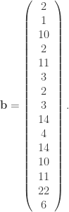
${\bf b}= \left(\begin{array}{c} 2 \\ 1 \\ 10 \\ 2 \\ 11 \\ 3 \\ 2 \\ 3 \\ 14 \\ 4 \\ 14 \\ 10 \\ 11 \\ 22 \\ 6 \\ \end{array}\right).$

The Massey ranking of these teams is a vector ${\bf r}$ which best fits the equation

$M{\bf r}={\bf b}.$

While the corresponding linear system is over-determined, we can look for a best (in the least squares sense) approximate solution using the orthogonal projection formula

$P_V = B(B^tB)^{-1}B^t,$

valid for matrices $B$ with linearly independent columns. Unfortunately, in this case $B=M$ does not have linearly independent columns, so the formula doesn’t apply.

Massey’s clever idea is to solve

$M^tM{\bf r}=M^t{\bf b}$

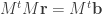
by row-reduction and determine the rankings from the parameterized form of the solution. To this end, we compute

$M^tM= \left(\begin{array}{rrrrrr} 5 & -1 & -1 & -1 & -1 & -1 \\ -1 & 5 & -1 & -1 & -1 & -1 \\ -1 & -1 & 5 & -1 & -1 & -1 \\ -1 & -1 & -1 & 5 & -1 & -1 \\ -1 & -1 & -1 & -1 & 5 & -1 \\ -1 & -1 & -1 & -1 & -1 & 5 \end{array}\right)$

and

$M^t{\bf b}= \left(\begin{array}{r} -24 \\ -10 \\ 10 \\ -29 \\ -10 \\ 63 \\ \end{array}\right).$

Then we compute the rref of

$A= (M^tM,M^t{\bf b}) = \left(\begin{array}{rrrrrr|r} 5 & -1 & -1 & -1 & -1 & -1 & -24 \\ -1 & 5 & -1 & -1 & -1 & -1 & -10 \\ -1 & -1 & 5 & -1 & -1 & -1 & 10 \\ -1 & -1 & -1 & 5 & -1 & -1 & -29 \\ -1 & -1 & -1 & -1 & 5 & -1 & -10 \\ -1 & -1 & -1 & -1 & -1 & 5 & 63 \end{array}\right),$

which is

$rref(M^tM,M^t{\bf b})= \left(\begin{array}{rrrrrr|r} 1 & 0 & 0 & 0 & 0 & -1 & -\frac{87}{6} \\ 0 & 1 & 0 & 0 & 0 & -1 & -\frac{73}{6} \\ 0 & 0 & 1 & 0 & 0 & -1 & -\frac{53}{6} \\ 0 & 0 & 0 & 1 & 0 & -1 & -\frac{92}{3} \\ 0 & 0 & 0 & 0 & 1 & -1 & -\frac{73}{6} \\ 0 & 0 & 0 & 0 & 0 & 0 & 0 \end{array}\right).$

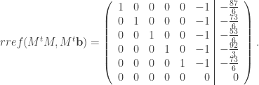
If ${\bf r}=(r_1,r_2,r_3,r_4,r_5,r_6)$ denotes the rankings of Army, Bucknell, Holy Cross, Lafayette, Lehigh, Navy, in that order, then

$r_1=r_6-\frac{87}{6},\ \ r_2=r_6-\frac{73}{6},\ \ r_3=r_6-\frac{53}{6},\ \ r_4=r_6-\frac{92}{6},\ \ r_5=r_6-\frac{73}{6}.$

Therefore

Lafayette $<$ Army = Bucknell = Lehigh $<$ Holy Cross $<$ Navy.

If we use this ranking to predict win/losses over the season, it would fail to correctly predict Army vs Holy Cross (Army won), Bucknell vs Lehigh, and Lafayette vs Army. This gives a prediction failure rate of $20\%$ .

Simple unsolved math problem, 6

Posted on 2016/12/01 by wdjoyner

If you know a little point-set topology, below is an unsolved math problem whose statement is relatively simple.

Probably everyone has at least seen the Mandelbrot set in some form, as it’s a popular object of mathematical artists. Here’s a picture from Wikipedia:

wikipedia_mandelbrot-set

The formal definition is as follows. Let $f_c (z)=z^2+c$ , where $c\in \mathbb{C}$ is a complex number. The Mandelbrot set $X$ is the complex plot of the set of complex numbers $c$ for which the sequence of iterates

$f_c (0), f_c (f_c (0)), f_c (f_c (f_c (0))), \dots,$

remains bounded in absolute value.
We say $X$ is locally connected if every point $x\in X$ admits a neighborhood basis consisting entirely of open, connected sets.

Conjecture: The Mandelbrot set $X$ is locally connected.

Yet Another Mathblog

Monthly Archives: December 2016