This is the fourth of a series of expository posts on matrix-theoretic sports ranking methods. This post discusses the Elo rating.
This system was originally developed by Arpad Elo (Elo (1903-1992) was a physics professor at Marquette University in Milwaukee and a chess master, eight-time winner of the Wisconsin State Chess Championships.) Originally, it was developed for rating chess players in the 1950s and 1960s. Now it is used for table tennis, basketball, and other sports.
We use the following version of his rating system.
As above, assume all the $n$ teams play each other (ties allowed)
and let 


Let 
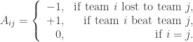
Let 
As in the previous post, the matrix 
- Initialize all the ratings to be
:
.
- After Team
, update their rating using the formula
where
and

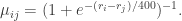
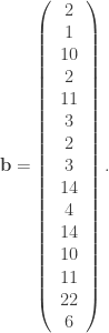
In the example of the Patriot league, the ratings vector is

This gives the ranking
Lafayette 
This gives a prediction failure rate of 
Some SageMath code for this:
def elo_rating(A):
    """
    A is a signed adjacency matrix for a directed graph.

    Returns elo ratings of the vertices of Gamma = Graph(A)

    EXAMPLES:
        sage: A = matrix(QQ,[
        [0 , -1 , 1  , -1 , -1 , -1 ],
        [1,   0 ,  -1,  1,  1,   -1  ],
        [-1 , 1 ,  0 ,  1 , 1  , -1  ],
        [1 , -1 , -1,  0 ,  -1 , -1  ],
        [1 , - 1 , - 1 , 1 , 0 , - 1  ],
        [1 ,  1  ,  1  , 1  , 1  , 0 ]
        ])
        sage: elo_rating(A)
        (85.124, 104.79, 104.88, 85.032, 94.876, 124.53)

    """
    n = len(A.rows())
    RR = RealField(prec=20)
    V = RR^n
    K = 10
    r0 = 100 # initial rating
    r = n*[r0]
    for i in range(n):
        for j in range(n):
            if ij and A[i][j]==1:
                S = 1
            elif ij and A[i][j]==-1:
                S = 0
            else:
                S = 1/2
            mu = 1/(1+e^(-(r[i]-r[j])/400))
            r[i] = r[i]+K*(S-mu)
    return V(r)

 (regarded as a weighted adjacency matrix) is in the figure below.

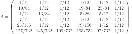
 by
by  , where
  is the
  doubly stochastic matrix with every entry equal to
  :
:

 (by reverse, I mean that the vector ranks the teams from worst-to-best, not from best-to-worst, as we have seen in previous ranking methods).


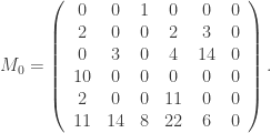
 be a non-negative square matrix determined by the results of their games, called the preference matrix. In his 1993 paper, Keener defined the score of the
 denotes the total number of games played by team
  is the rating vector (where
  denotes the rating of team
 so we ignore the
  factor.)
 is proportional to its score. The score is expressed as a matrix product
  , where
  such that
  , for each
  .
. has an eigenvector
  having positive entries associated to the largest eigenvalue $\lambda_{max}$ of
  . Indeed,
  , of multiplicity
 .
. , and the total runs allowed by team
  . Here, we order the six teams as above (team
  is Bucknell, and so on). For instance if X played Y and the scores were
  ,
,  ,
,  in the position of row X and column Y.
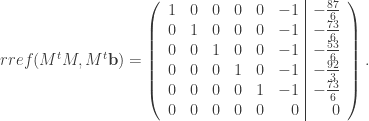
 matrix:


 with linearly independent columns. Unfortunately, in this case
  does not have linearly independent columns, so the formula doesn’t apply.
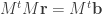


 .
.
You must be logged in to post a comment.