According to [1], a sestina is a highly structured poem consisting of six six-line stanzas followed by a tercet (called its envoy or tornada), for a total of thirty-nine lines. The same set of six words ends the lines of each of the six-line stanzas, but in a shuffled order each time. The shuffle used is very similar to the Mongean shuffle.
Define 


Theorem: If p is an n-cycle then 2n+1 is a prime.
Call such a prime a “sestina prime”. Which primes are sestina primes?
Here is Python/Sage code for this permutation:
def sestina(n):
    """
    Computes the element of the symmetric group S_n associated to the shuffle above.

    EXAMPLES:
        sage: sestina(4)
        (1,2,4)
        sage: sestina(6)
        (1,2,4,5,3,6)
        sage: sestina(8)
        (1,2,4,8)(3,6,5,7)
        sage: sestina(10)
        (1,2,4,8,5,10)(3,6,9)
        sage: sestina(12)
        (1,2,4,8,9,7,11,3,6,12)(5,10)
        sage: sestina(14)
        (1,2,4,8,13,3,6,12,5,10,9,11,7,14)
        sage: sestina(16)
        (1,2,4,8,16)(3,6,12,9,15)(5,10,13,7,14)
        sage: sestina(18)
        (1,2,4,8,16,5,10,17,3,6,12,13,11,15,7,14,9,18)
        sage: sestina(20) (1,2,4,8,16,9,18,5,10,20)(3,6,12,17,7,14,13,15,11,19)
        sage: sestina(22) (1,2,4,8,16,13,19,7,14,17,11,22)(3,6,12,21)(5,10,20)(9,18)

    """
    def fcn(k, n):
        if k<=int(n/2):
            return 2*k
        else:
            return 2*n+1-2*k
    L = [fcn(k,n) for k in range(1,n+1)]
    G = SymmetricGroup(n)
    return G(L)
And here is an example due to Ezra Pound [3]:
                                  I

Damn it all! all this our South stinks peace.
You whoreson dog, Papiols, come! Let’s to music!
I have no life save when the swords clash.
But ah! when I see the standards gold, vair, purple, opposing
And the broad fields beneath them turn crimson,
Then howl I my heart nigh mad with rejoicing.

                                     II

In hot summer have I great rejoicing
When the tempests kill the earth’s foul peace,
And the light’nings from black heav’n flash crimson,
And the fierce thunders roar me their music
And the winds shriek through the clouds mad, opposing,
And through all the riven skies God’s swords clash.

                                     III

Hell grant soon we hear again the swords clash!
And the shrill neighs of destriers in battle rejoicing,
Spiked breast to spiked breast opposing!
Better one hour’s stour than a year’s peace
With fat boards, bawds, wine and frail music!
Bah! there’s no wine like the blood’s crimson!

                                     IV

And I love to see the sun rise blood-crimson.
And I watch his spears through the dark clash
And it fills all my heart with rejoicing
And prys wide my mouth with fast music
When I see him so scorn and defy peace,
His lone might ’gainst all darkness opposing.

                                     V

The man who fears war and squats opposing
My words for stour, hath no blood of crimson
But is fit only to rot in womanish peace
Far from where worth’s won and the swords clash
For the death of such sluts I go rejoicing;
Yea, I fill all the air with my music.

                                     VI

Papiols, Papiols, to the music!
There’s no sound like to swords swords opposing,
No cry like the battle’s rejoicing
When our elbows and swords drip the crimson
And our charges ’gainst “The Leopard’s” rush clash.
May God damn for ever all who cry “Peace!”

                                     VII

And let the music of the swords make them crimson
Hell grant soon we hear again the swords clash!
Hell blot black for always the thought “Peace”!
References:
[1] http://en.wikipedia.org/wiki/Sestina
[2] Richard Dore and Anton Geraschenko,”Sestinas and Primes” posted to http://stacky.net/wiki/index.php?title=Course_notes, and http://math.berkeley.edu/~anton/written/sestina.pdf
[3] Ezra Pound, “Sestina: Altaforte” (1909), (originally published int the English Review, 1909)
[4] John Bullitt, N. J. A. Sloane and J. H. Conway , http://oeis.org/A019567
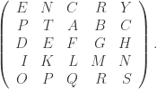
 be the binary Hamming [7,4,3] code defined by the generator matrix
 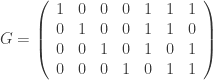 and check matrix
 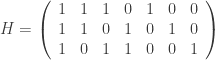 . In other words, this code is the row space of G and the kernel of H. We can enter these into Sage as follows:
 defined by
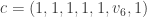
  . Using this map, the codewords are easy to describe and enumerate:
 .
. . This must be a codeword (no lies) or differ from a codeword by exactly one bit (1 lie). In either case, you can find n by decoding this vector.
 .
. in region i of the Venn diagram.


 , for some unknown
  . We solve for this unknown using the check vertex equation
  . The decoded codeword is
 . In this case, we know the vertices 9 and 10 fail, so
  . We solve using

 . By majority vote, we get
  .
.  is its length,
  is its dimension, and
  is its minimum distance),
  is a generating matrix,
  is a check matrix, and
  is the dual code of
  to be a cover, and the message
  we embed is an element of
  . Once we find a vector
  of lowest weight such that
  , we call
  the stegocover. The stegocover looks a lot like the original cover and “contains” the message m. This will be explained in more detai below.
 .
. with a fixed basis, where
  is an integer called the length of the code. Moreover, the basis for the ambient space
 are the rows of
 . The vector of coefficients,
  represents the information you want to encode and transmit.
 . This matrix is called a check matrix of
  matrix then a full rank check matrix
  matrix.
 is the generating matrix for
  is a parity check matrix.
 be an integer and let
  matrix whose columns are all the distinct non-zero vectors of
  , and let
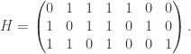
 entries is the identity matrix
  , the generator matrix
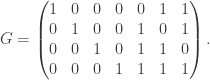
 is a subset of
  for some
  . Let
. Let  be a coset of
  .
.
 is a set of all possible covers
 is a set of all possible messages
 is a set of all possible keys
 is an embedding function
 is a recovery function

 ,
,  ,
,  . We will assume that a fixed key
  is called the plain cover,
  is called the stegocover. Let
  , where
  is a fixed integer such that
  .
.  and consider the cover
  . Regarded as a
  matrix,
 . First we compute the stegocover:
 ,
,  .
. is the matrix whose entries are
  ,
,  is a regular graph of degree wt(f), where wt denotes the Hamming weight of f when regarded as a vector of values (of length
  ).
). and its adjacency matrix A, the spectrum Spec(
 (this only makes sense if n is even). The Hadamard transform of a integer-valued function f is an integer-valued function over
 given by
  .
.
 given by
  .
.
 BTW, the
  analog is:
 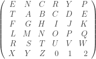 .
. case is in Alasdair’s book):
![[n,k,d]](https://s0.wp.com/latex.php?latex=%5Bn%2Ck%2Cd%5D&bg=ffffff&fg=323232&s=0&c=20201002) linear error correcting block code
linear error correcting block code  . A
. A  , where
  is the rank of M. Recall, a circuit in a matroid M=(E,J) is a minimal dependent subset of E — that is, a dependent set whose proper subsets are all independent (i.e., all in J).
  matrix
  . The vector matroid M=M[H] is a matroid for which the smallest sized dependency relation among the columns of H is determined by the check relations
  , where
  is a codeword (in C which has minimum dimension d). Such a minimum dependency relation of H corresponds to a circuit of M=M[H].
You must be logged in to post a comment.