This post shall explain how the F5 stegosystem (in a simple case) can be implemented in Sage. I thank Carlos Munuera for teaching me these ideas and for many helpful conversations on this matter. I also thank Kyle Tucker-Davis [1] for many interesting conversations on this topic.
Steganography, meaning “covered writing,” is the science of secret communication [4]. The medium used to carry the information is called the “cover” or “stego-cover” (depending on the context – these are not synonymous terms). The term “digital steganography” refers to secret communication where the cover is a digital media file.
One of the most common systems of digital steganography is the Least Significant Bit (LSB) system. In this system, we assume the “cover” image is represented as a finite sequence of binary vectors of a given length. In other words, a greyscale image is regarded as an array of pixels, where each pixel is represented by a binary vector of a certain fixed length. Each such vector represents a pixel’s brightness in the cover image. The encoder embeds (at most) one bit of information in the least significant bit of eaach vector. Care must be taken with this system to ensure that the changes made do not betray the stego-cover, while still maximizing the information hidden.
From a short note of Crandell [3] in 1998, it was realized that error-correcting codes can give rise to “stego-schemes”, ie, methods by which a message can be hidden in a digital file efficiently.
Idea in a nutshell: If 


(This particular scheme is called the F5 stegosystem, and is due to Westfeld.)
Quick background on error-correcting, linear, block codes [5]
A linear error-correcting block code is a finite dimensional vector space over a finite field with a fixed basis. We assume the finite field is the binary field 
We shall typically think of a such a code as a subspace 


There are two common ways to specify a linear code
-
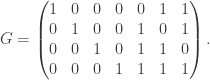
You can give
the rows of a matrix called a generator matrix
affect the code itself.If
are the rows of
is the set of linear combinations of the row vectors
. The vector of coefficients,
represents the information you want to encode and transmit.
In other words, encoding of a message can be defined via the generator matrix:
-
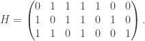
You can give
. This matrix is called a check matrix of


Note that if 

These two ways of defining a code are not unrelated.
Fact:
If 

Exaample:
Let 

Let 
In this form, namely when the columns of 

A coset of 


a coset leader of
Fact:
The coset leaders of a Hamming code are those vectors of 
Steganographic systems from error-correcting codes
This section basically describes Crandell’s idea [3] in a more formalized language.
Following Munuera’s notation in [6], a steganographic system
where

-
is a set of all possible covers
-
is a set of all possible messages
-
is a set of all possible keys
-
is an embedding function
-
is a recovery function
and these all satisfy

for all 


the dependence on an element in the keyspace 


Sage examples
How do we compute the emb map?
We need the following Sage function.
def hamming_code_coset_leader(C, y):
      """
      Finds the coset leader of a binary Hamming code C.
      EXAMPLES:
      """
      F = C.base_ring()
      n = C.length()
      k = C.dimension()
      r = n-k
      V0 = F^r
      if not(y in V0):
          RaiseError, "Input vector is not a syndrome."
      H = C.check_mat()
      colsH = H.columns()
      i = colsH.index(y)
      V = F^n
      v = V(0)
      v[i] = F(1)
      return v
Let 


V = GF(2)^(63)
rhino = V([1,1,1,1,1,1,1,1,1,
           1,1,1,1,1,1,1,1,1,
           1,1,1,1,0,0,1,1,1,
           1,0,0,0,0,0,0,1,1,
           1,0,0,0,0,0,0,0,1,
           1,0,0,0,0,0,0,1,1,
           1,0,0,1,1,0,0,1,1])
A = matrix(GF(2),7,rhino.list())
matrix_plot(A)
this looks like an elephant or a rhino:

Now we embed the message 
C = HammingCode(6,GF(2))
H = C.check_mat()
V0 = GF(2)^6
m = V0([1,0,1,0,1,0])
z = hamming_code_coset_leader(C, m)
stegocover = rhino+z
A = matrix(GF(2),7,stegocover.list())
matrix_plot(A)
It looks like another rhino/elephant:

Note only one bit is changed since the Hamming weight of z is at most 1. To recover the message m, just multiply the vector “stegocover” by H.
That’s how you can use Sage to understand the F5 stegosystem, at least in a very simple case.
REFERENCES:
[1] Kyle Tucker-Davis, “An analysis of the F5 steganographic system”, Honors Project 2010-2011
http://www.usna.edu/Users/math/wdj/tucker-davis/
[2] J. Bierbrauer and J. Fridrich. “Constructing good covering codes for applications in Steganography}. 2006.
http://www.math.mtu.edu/jbierbra/.
[3] Crandall, Ron. “Some Notes on Steganography”. Posted on a Steganography Mailing List, 1998.
http://os.inf.tu-dresden.de/westfeld/crandall.pdf
[4] Wayner, Peter. Disappearing Cryptography. Morgan Kauffman Publishers. 2009.
[5] Hill, Raymond. A First Course in Coding Theory. Oxford University Press. 1997.
[6] Munuera, Carlos. “Steganography from a Coding Theory Point of View”. 2010.
http://www.singacom.uva.es/oldsite/Actividad/s3cm/s3cm10/10courses.html
[7] Zhang, Weiming and S. Li. “Steganographic Codes- a New Problem of Coding Theory”. preprint, 2005.
http://arxiv.org/abs/cs/0505072.
 ,
,  .
. is the matrix whose entries are
  ,
,  is a regular graph of degree wt(f), where wt denotes the Hamming weight of f when regarded as a vector of values (of length
  ).
). and its adjacency matrix A, the spectrum Spec(
 (this only makes sense if n is even). The Hadamard transform of a integer-valued function f is an integer-valued function over
 given by
  .
.
 given by
  .
.
 equal to the New Year.
 BTW, the
  analog is:
 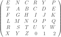 .
. case is in Alasdair’s book):


You must be logged in to post a comment.