Searching with lies, 1

Posted on 2012/06/19 by wdjoyner

In Stanislaw Ulam’s 1976 autobiography (Adventures of a mathematician, Scribner and Sons, New York, 1976), one finds the following problem concerning two players playing a generalization of the childhood game of “20 questions”.
(As a footnote: the history of who invented this game is unclear. It occurred in writings of Renyi, for example “On a problem in information theory” (Hungarian), Magyar Tud. Akad. Mat. Kutató Int. Közl. 6 (1961)505–516, but may have been known earlier under the name “Bar-kochba”.)

Problem: Player 1 secretly chooses a number from $1$ to $M$ ( $M$ is large but fixed, say $M = 1000000$ ). Player 2 asks a series of “yes/no questions” in an attempt to determine that number. Player 1 can lie at most $e$ times ( $e\geq 0$ is fixed). Assuming best possible play on both sides, what is the minimum number of “yes/no questions” Player 2 must ask to (in general) be able to correctly determine the number Player 1 selected?

There is a very large literature on this problem. Just google “searching with lies” (with the quotes) to see a selection of the papers (eg, this paper). It turns out this children’s game, when suitably generalized, has numerous applications to computer science and engineering.

We start with a simple example. Pick an integer from 0 to 1000000. For example, suppose you pick $2^{19}+1 = 524289$ .

Here is how I can ask you 20 True/False questions and guess your number.

Is your number less than 524288? False

Is your number less than 655360? True
Is your number less than 589824? True

Is your number less than 557056? True
Is your number less than 540672? True
Is your number less than 532480? True
Is your number less than 528384? True
Is your number less than 526336? True
Is your number less than 525312? True
Is your number less than 524800? True
Is your number less than 524544? True
Is your number less than 524416? True
Is your number less than 524352? True
Is your number less than 524320? True
Is your number less than 524304? True
Is your number less than 524296? True
Is your number less than 524292? True
Is your number less than 524290? True
Is your number less than 524289? False

This is the general description of the binary search strategy:
First, divide the whole interval of size $2^{20}$ into half and find which half the number lies in. Discard the one it does not lie in.
Second, divide the subinterval of size $2^{19}$ into half and find which half the number lies in. Discard the one it does not lie in.
Third, divide the subinterval of size $2^{18}$ into half and find which half the number lies in. Discard the one it does not lie in.
And so on.
This process must stop after 20 steps, as you run out of non-trivial subintervals.

This is an instance of “searching with lies” where no lies are told and “feedback” is allowed.

Another method:
I don’t know what your number is, but whatever it is, represent it in binary as a vector

$b = (b_0, b_1, ..., b_N)\ \ {\rm so}\ \ M = b_02^0 + b_12^1 + ... + b_N2^N,$

where $N = ceiling(\log_2(N))=20$ , where $2^{20}-1 = 1048574$ . The 20 questions are:
Is $b_0 = 0$ ?
Is $b_1 = 0$ ?
and so on
Is $b_N = 0$ ?
You may determine the value of the $b_i$ ‘s from this (since each $b_i$ is either 0 or 1).

This is an instance of “searching with lies” where no lies are told and “feedback” is not allowed.

Let’s go back to our problem where Player 1 secretly chooses a number from $1$ to $M$ ( $M$ is large but fixed, say $M = 1000000$ ). Use the following notation: If the answers between successive questions is possible and then questions may be adapted to these answers (“feedback allowed”), call this minimum number of “yes/no questions” Player 2 must ask, $f(M,e)$ . If feedback is not allowed, call this minimum number $g(M,e)$ .

Clearly, $f(M,e)\leq g(M,e).$

In practice, we not only want to know $f(M,e)$ (resp., $g(M,e$ ) but an efficient algorithm for determining the “yes/no questions” Player 2 should ask.

In his 1964 PhD thesis (E. Berlekamp, Block coding with noiseless feedback, PhD Thesis, Dept EE, MIT, 1964), Berlekamp was concerned with a discrete analog of a problem which arises when trying to design a analog-to-digital converter for sound recording which compensates for possible feedback.

To formulate this problem in the case when lies are possible, we introduce some new terms.

Definitions

A binary code is a set $C$ of $n$ -tuples of $0$ ‘s and $1$ ‘s, i.e., a subset $C\subset GF(2)^n$ , where $GF(2)={\bf Z}/2{\bf Z}=\{0,1\}$ is the field of integers $\pmod{2}$ . If we assume, in addition, $C$ is a vector space over $GF(2)$ then we say $C$ is a linear binary code. A codeword is an element of a binary code.
The Hamming distance between $n$ -tuples $w,w'\in GF(2)^n$ is the number $d(w,w')$ of non-zero coordinates of $w-w'$ .
The minimum distance of $C$ is the smallest integer $d$ such that $d(c,c')\geq d$ for all distinct $c,c'\in C$ .

For example, let

$C = \{ (0, 0, 0), (1, 1, 1) \} \subset GF(2)^2.$

This is a 1-error correcting code of minimum distance $d=3$ .

We say that $C$ is $e$ -error correcting if the following property always holds: given any $w\in GF(2)^n$ and any $c\in C$ , if $d(w,c)\leq e$ then every $c'\in C$ , $c\not= c'$ , must satisfy $d(w,c')\ge e$ (in other words, there is at most one codeword within distance $e$ from any $w\in GF(2)^n$ ).

Let $A(n,d)$ denote the largest possible size of a binary code $C\subset GF(2)^n$ of minimum distance $d$ .

Fact: If a binary code $C\subset GF(2)^n$ is $e$ -error correcting then $|C|\leq A(n,2e+1)$ .

Let $B(n,d)$ denote the largest possible size of a binary linear code $C\subset GF(2)^n$ of minimum distance $d$ . It is known that $B(n,d)=2^k$ , for some $k$ (called the dimension of $C$ ).

Clearly, $A(n,d)\leq B(n,d)$ .

A Reduction

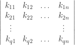
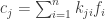
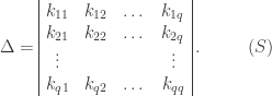
Fact: Fix any $e$ and $M$ . $g(M,e)$ is the smallest $n$ such that $A(n,2e+1)\geq M$ .

Record the $n$ answers to all the “yes/no questions” as an $n$ -tuple of $0$ ‘s (for “no”) and $1$ ‘s (for “yes”). The binary code $C$ is the set of all codewords corresponding to correct answers. Intuitively, if you are Player 2 and you ask Player 1 what the coordinates of his codeword $c$ associated to his secret number is, and if he lies $e$ times then you will receive from him a binary vector $w$ of Hamming distance $e$ from a codeword. Since $C$ is $e$ -error correcting, you can determine $c$ from $w$ .

We want the smallest possible $n$ satisfying the condition $A(n,2e+1)\geq M$ . The values of $B(n,2e+1)$ (or $\log_2 B(n, d)$ , where we take $d=2e+1$ , to be more precise) have been tabulated for “small” values of $M$ and $e$ online at the MinT website (U. of Salzburg, Wolfgang Ch. Schmid and Rudolf Schürer), codetables.de (Markus Grassl), and Boston U. (Ari Trachtenberg). This gives us an upper bound for $g(M,e)$ , and hence also for $f(M,e)$ for “small” values of $M$ and $e$ .

Here’s a recipe for using online tables to find a good upper bound the smallest number Q of questions Player 2 must ask Player 1, if Player 1 gets to lie $e$ times:

Find the smallest k such that $2^k \geq M$ ,
go to the table minT and go to the row $d=2e+1$ ; find the smallest column number n which contains an entry greater than or equal to k.
that column number n is an upper bound for Q.

Lester Hill’s “The checking of the accuracy …”, part 7

Posted on 2012/06/09 by wdjoyner

Backstory: Lester Saunders Hill wrote unpublished notes, about 40 pages long, probably in the mid- to late 1920s. They were titled “The checking of the accuracy of transmittal of telegraphic communications by means of operations in finite algebraic fields”. In the 1960s this manuscript was given to David Kahn by Hill’s widow. The notes were typewritten, but mathematical symbols, tables, insertions, and some footnotes were often handwritten. I thank Chris Christensen, the National Cryptologic Museum, and NSA’s David Kahn Collection, for their help in obtaining these notes. Many thanks also to Rene Stein of the NSA Cryptologic Museum library and David Kahn for permission to publish this transcription. Comments by transcriber will look his this: [This is a comment. – wdj]. I used Sage (www.sagemath.org) to generate the tables in LaTeX.

Here is just the seventh section of his paper. I hope to post more later. (Part 6 is here.)

Section 7: The general form of reference matrix

Let $a_1, a_2, \dots a_n$ be $n$ different elements of our finite field $F$ , and let $a_i$ be different from the zero element of $F$ . Then we shall emply a reference matrix of the form

$Q = \left( \begin{array}{cccc} a_1 & a_2 & \dots & a_{n} \\ a_1^2 & a_2^2 & \dots & a_{n}^2 \\ \vdots & & & \vdots \\ a_1^q & a_2^q & \dots & a_{n}^q \\ \end{array} \right)$

or of the form

$Q' = \left( \begin{array}{cccc} 1 & 1 & \dots & 1 \\ a_1 & a_2 & \dots & a_{n} \\ a_1^2 & a_2^2 & \dots & a_{n}^2 \\ \vdots & & & \vdots \\ a_1^{q-1} & a_2^{q-1} & \dots & a_{n}^{q-1} \\ \end{array} \right) \, .$

The actual procedure involved, and the real equivalence for checking purposes, of $Q$ and $Q'$ , will presently be illustrated. We note here merely that each of the matrices $Q$ , $Q'$ is of index $q$ . Let us examine $Q'$ . A similar argument will be applicable to $Q$ .

Suppose, for argument, that $Q'$ contains a vanishing $q$ -rowed determinant. Without loss of generality, we suppose that it is

$Q' = \left| \begin{array}{cccc} 1 & 1 & \dots & 1 \\ a_1 & a_2 & \dots & a_{q} \\ a_1^2 & a_2^2 & \dots & a_{q}^2 \\ \vdots & & & \vdots \\ a_1^{q-1} & a_2^{q-1} & \dots & a_{q}^{q-1} \\ \end{array} \right| \, .$
Since this determinant is equal to zero, Lemma 4 guarantees the existence, in our field $F$ , of the elements

$\lambda_1, \lambda_2, \dots \lambda_q,$

not all equal to zero, for which we may write

$\lambda_1 + \lambda_2 a_i +\lambda_3 a_i^2 + \dots + \lambda_q a_q^{q-1} = 0,$
( $i=1,2, \dots, q$ ). The $a_i$ being, as assumed, all different, this implies that the equation

$\lambda_1 + \lambda_2 x +\lambda_3 x^2 + \dots + \lambda_q x^{q-1} = 0,$

has $q$ different roots in $F$ , an implication which contradicts Lemma 5.

Thus $Q'$ contains no vanishing $q$ -rowed determinant, and if of index $q$ . In the same way, $Q$ may be shown to be of index $q$ . But unless these matrices are constructed with care, they will, of course, generally contain vanishing determinants of various orders less than $q$ . We defer for the moment the further consideration of this matter.

Lester Hill’s “The checking of the accuracy …”, part 6

Posted on 2012/06/09 by wdjoyner

Backstory: Lester Saunders Hill wrote unpublished notes, about 40 pages long, probably in the mid- to late 1920s. They were titled “The checking of the accuracy of transmittal of telegraphic communications by means of operations in finite algebraic fields”. In the 1960s this manuscript was given to David Kahn by Hill’s widow. The notes were typewritten, but mathematical symbols, tables, insertions, and some footnotes were often handwritten. The manuscript is being LaTeXed “as we speak”. I thank Chris Christensen, the National Cryptologic Museum, and NSA’s David Kahn Collection, for their help in obtaining these notes. Many thanks also to Rene Stein of the NSA Cryptologic Museum library and David Kahn for permission to publish this transcription. Comments by transcriber will look his this: [This is a comment. – wdj]. I used Sage (www.sagemath.org) to generate the tables in LaTeX.

Here is just the sixth section of his paper. I hope to post more later. (Part 5 is here.)

Section 6: Arbitrary distrbution of errors affecting the $f_i$ and the $c_j$

It is highly desirable, although not strictly necessary, to fashion the reference matrix $Q$ in such a manner that every determinant contained in it, of every order, be different from zero.

Reference matrices of a practical type, and without a vanishing determinant of any order, may be construted in certain finite fields $F$ by very direct methods which can be more easily illustrated than described. It will be expedient at this poin, even at the expense of breaking the continuity of our discussion, to introduce concrete examples of operations in finite fields, and to show how reference matrices be conveniently set up in particular cases. The desirability of contriving that such matrices contain no vanishing determinant can then be brought out more effectively. The examination of arbitrary distributions of errors among the $n+q$ elements of a telegraphic sequence

$f_1, f_2, \dots, f_n, c_1, c_2, \dots, c_q$

can be deferred, therefore, until later.

But, before going into details, we will describe the general form of reference matrix to be employed in all cases.

Lester Hill’s “The checking of the accuracy …”, part 5

Posted on 2012/06/09 by wdjoyner

Backstory: Lester Saunders Hill wrote unpublished notes, about 40 pages long, probably in the mid- to late 1920s. They were titled “The checking of the accuracy of transmittal of telegraphic communications by means of operations in finite algebraic fields”. In the 1960s this manuscript was given to David Kahn by Hill’s widow. The notes were typewritten, but mathematical symbols, tables, insertions, and some footnotes were often handwritten. The manuscript is being LaTeXed “as we speak”. I thank Chris Christensen, the National Cryptologic Museum, and NSA’s David Kahn Collection, for their help in obtaining these notes. Many thanks also to Rene Stein of the NSA Cryptologic Museum library and David Kahn for permission to publish this transcription. Comments by transcriber will look his this: [This is a comment. – wdj]. I used Sage (www.sagemath.org) to generate the tables in LaTeX.

Here is just the fifth section of his paper. I hope to post more later. (Part 4 is here.)

Section 5: The error distribution with at least $q$ errors $\epsilon_i$

Let the sequence (footnote: Arbitrary error distributions will be considered later. Cf. sections 15-18.)

$f_1, f_2, \dots, f_n,\ c_1, c_2, \dots, c_q$
be transmitted in the form

$f_1', f_2', \dots, f_n',\ c_1', c_2', \dots, c_q' \, ,$
containing $t\geq q$ errors which affect the $f_i$ , and $h\geq 0$ errors which affect the $c_j$ .

Let $t=q+s$ . Then, to avoid discussing again the case already considered, we assume that at least one of the two integers $s, h$
is greater than $0$ .

Let the errors among the $c_j$ be $\delta_{j_1}, \delta_{j_2}, \dots , \delta_{j_h}$ , affecting the $c_{j_1}, c_{j_2}, \dots , c_{j_h}$ . Without loss in generality, we may assume that the $t$ errors affecting the $f_i$ are $\epsilon_1, \epsilon_2, \dots, \epsilon_t$ , so that the first $t$ of the $f_i$ are transmitted in error.

Suppose that the mutilated sequence is in full check. Then:

$\sum_{i=1}^t k_{ji}(f_i+\epsilon_i)+\sum_{i=t+1}^n k_{ji}f_i =c_j+\delta_j$

$\sum_{i=1}^n k_{ji}f_i+\sum_{i=1}^t k_{ji}\epsilon_i =c_j+\delta_j$

whence

$\sum_{i=1}^t k_{ji}\epsilon_i=\delta_j$

where $j=1,2,\dots, q$ and where $\delta_j$ in $c_j$ and may, of course, be
equal to $0$ .

It follows that

$\sum_{i=1}^q k_{ji}\epsilon_i = \delta_j - \sum_{i=1}^t k_{ji}\epsilon_i = b_j = \phi_j(\epsilon_{q+1}, \epsilon_{q+2}, \dots , \epsilon_t, \delta_j),$
where $j=1,2,\dots, q$ and where $\phi_j$ denotes a polynomial in the errors $\epsilon_{q+1}, \epsilon_{q+2}, \dots , \epsilon_t, \delta_j$ .

The index of the reference matrix being $q$ , the determinant

$\left| \begin{array}{cccc} k_{11} & k_{12} & \dots & k_{1n} \\ k_{21} & k_{22} & \dots & k_{2n} \\ \vdots & & & \vdots \\ k_{q1} & k_{q2} & \dots & k_{qn} \\ \end{array} \right|$

of the systems of equations

$\sum_{i=1}^q k_{ji}\epsilon_i = b_j \ \ \ \ \ \ \ \ \ \ (j=1,2,\dots, q)$

is not zero. Hence if all the $b_j$ are equal to zero, Lemma 1 demands that all the $\epsilon_i$ , for $i=1, 2, \dots, q$ , be equal to zero, contrary to hypothesis.

If at least one of the $b_j$ is different from $0$ , Lemma 3 shows that $\epsilon_{1}, \epsilon_{2}, \dots , \epsilon_q$ are uniquely determined as functions of the $b_j$ , and therefore as functions of $\epsilon_{q+1}, \epsilon_{q+2}, \dots , \epsilon_t, \delta_1, \delta_2, \dots, \delta_q$ :

$\epsilon_i = \xi_i (\epsilon_{q+1}, \epsilon_{q+2}, \dots , \epsilon_t, \delta_1, \delta_2, \dots, \delta_q),\ \ \ \ \ \ \ \ \ \ (j=1,2,\dots, q)$

the functions $\xi_i$ being, of course, rational functions. But, by assumption, all of the $\delta_j$, except $\delta_{j_1}, \dots, \delta_{j_h}$ , vanish. Hence $\epsilon_i$ ( $i=1,2,\dots, q$ ) is a rational function of $\epsilon_{q+1}, \epsilon_{q+2}, \dots , \epsilon_t, \delta_{j_1}, \delta_{j_2}, \dots, \delta_{j_h}$ .

We conclude that if the mutilated message, containing $t+h$ errors, is to check up, so that the presence of error can escape detection, $q$ of the errors must be carefully adjusted as rational functions of the remaining $t+h-q$ errors.

It is easy to measure the chance that mere accidents of erroneous telegraphic transmittal might effect this adjustment. Let $\Gamma$ denote the total number of elements in the finite algebraic field $F$ which we are dealing. When an error is made in transmitting a sequence of elements of $F$ , the error may evidently have any one of $\Gamma -1$ values — an error with the value $0$ being no real error at all. It is therefore clear that our set of $t+h$ errors will enjoy only $1$ chance in $(\Gamma -1)^q$ of being accidentally adjusted so as to escape detection.

When $t=q+s$ errors occur among the $f_i$ and $h$ errors occur among the $c_j$ in the transmittal of the sequence $f_1, f_2, \dots, f_n,\ c_1, c_2, \dots, c_q$ , the errors being all of accidental telegraphic origin, the presence of error will infallibly be disclosed if $h=s=0$ ; and will enjoy a $1$ -in- $(\Gamma -1)^q$ of escaping disclosure if either of the two integers $h$ , $s$ is greater than $0$ .

This statement summarizes the results of the present section and those of section 4.

Lester Hill’s “The checking of the accuracy …”, part 4

Posted on 2012/06/09 by wdjoyner

Backstory: Lester Saunders Hill wrote unpublished notes, about 40 pages long, probably in the mid- to late 1920s. They were titled “The checking of the accuracy of transmittal of telegraphic communications by means of operations in finite algebraic fields”. In the 1960s this manuscript was given to David Kahn by Hill’s widow. The notes were typewritten, but mathematical symbols, tables, insertions, and some footnotes were often handwritten. The manuscript is being LaTeXed “as we speak”. I thank Chris Christensen, the National Cryptologic Museum, and NSA’s David Kahn Collection, for their help in obtaining these notes. Many thanks also to Rene Stein of the NSA Cryptologic Museum library and David Kahn for permission to publish this transcription. Comments by transcriber will look his this: [This is a comment. – wdj]. I used Sage (www.sagemath.org) to generate the tables in LaTeX.

Here is just the fourth section of his paper. I hope to post more later. (Part 3 is here.)

Section 4: Index of the reference matrix $Q$

There will be considerable advantage in employing a reference matrix $Q$ of index $q$ .

Consider the sequence $f_1, f_2, \dots, f_n, c_1, c_2, \dots, c_q$ which is to be transmitted.
Errors may be made in transmittal, and the sequence may come through in the form

$f_1', f_2', \dots, f_n', c_1', c_2', \dots, c_q'\, ,$

where $f_i'=f_i+\epsilon_i$ , $c_j' = c_j + \delta_j$ , where $i = 1, 2, \dots, n$ , $j = 1, 2, \dots, q$ , the errors $\epsilon_i$ and $\delta_j$ being, of course, elements of the finite field $F$ . If $f_i$ (resp., $c_j$ ) is correctly transmitted then the error $\epsilon_i$ (resp., $c_j$ ) vanishes, and $f_i'=f_i$ (resp., $c_j'=c_j$ ).

Let us consider what happens when out sequence is mutilated to the extent of $q$ errors, all of which affect the $f_i$ (the $c_j$ being supposed correctly transmitted).

There is no real loss of generality if we assume that the errors affect the first $q$ of the
$f_i$ , the errors being $\epsilon_1$ , $\epsilon_2, \dots, \epsilon_q$ . Since the $c_j$ have been correctly transmitted, the mutilated message can not be in check unless

$c_j = \sum_{i=1}^q k_{ji}(f_i+\epsilon_i) +\sum_{i=q+1}^n k_{ji}f_i =\sum_{i=1}^n k_{ji}f_i + \sum_{i=1}^q k_{ji}\epsilon_i.$

But we recall that, by definition, $c_j =\sum_{i=1}^n k_{ji}f_i$ . Hence the message will fail to check, and the presence of error will be disclosed, unless the $q$ errors $\epsilon_i$ satisfy the system of equations

$\sum_{i=1}^q k_{ji}\epsilon_i = 0$

for $j = 1, 2, \dots, q$ , of which the determinant is

$\Delta = \begin{array}{|cccc|} k_{11} & k_{12} & \dots & k_{1q} \\ k_{21} & k_{22} & \dots & k_{2q} \\ \vdots & & & \vdots \\ k_{q1} & k_{q2} & \dots & k_{qq} \\ \end{array} \, . \ \ \ \ \ \ \ \ (S)$

But our matrix is supposed to be of index $q$ , so that $\Delta \not=0$. It follows, by Lemma 1, that the system (S) has no solution other than $\epsilon_i=0$ , for $i=1,2,\dots, q$ . Hence $q$ errors, confined to the $f_i$ , can not escape disclosure if the reference matrix $Q$ is of index $q$ . By the same argument, applied a fortiori, a set of less than $q$ errors, confined to the $f_i$ , will certainly be disclosed when $Q$ is of index $q$ .

If the reference matrix $Q$ is of index $q$ , we can make the following statement:

Whenever the sequence $f_1, f_2, \dots, f_n, c_1, c_2, \dots, c_q$ is transmitted with errors not affecting the $c_i$ , and not more than $q$ in number, the presence of error will infallibly be disclosed.

We shall hereafter understand that $Q$ is of index $q$ .

Remarks on the Hamming [7.4.3] code and Sage

Posted on 2012/02/28 by wdjoyner

This post simply collects some very well-known facts and observations in one place, since I was having a hard time locating a convenient reference.

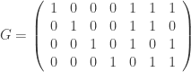Let $C$ be the binary Hamming [7,4,3] code defined by the generator matrix $G = \left(\begin{array}{rrrrrrr} 1 & 0 & 0 & 0 & 1 & 1 & 1 \\ 0 & 1 & 0 & 0 & 1 & 1 & 0 \\ 0 & 0 & 1 & 0 & 1 & 0 & 1 \\ 0 & 0 & 0 & 1 & 0 & 1 & 1 \end{array}\right)$ and check matrix 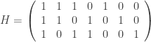$H = \left(\begin{array}{rrrrrrr} 1 & 1 & 1 & 0 & 1 & 0 & 0 \\ 1 & 1 & 0 & 1 & 0 & 1 & 0 \\ 1 & 0 & 1 & 1 & 0 & 0 & 1 \end{array}\right)$ . In other words, this code is the row space of G and the kernel of H. We can enter these into Sage as follows:

sage: G = matrix(GF(2), [[1,0,0,0,1,1,1],[0,1,0,0,1,1,0],[0,0,1,0,1,0,1],[0,0,0,1,0,1,1]])
sage: G
[1 0 0 0 1 1 1]
[0 1 0 0 1 1 0]
[0 0 1 0 1 0 1]
[0 0 0 1 0 1 1]
sage: H = matrix(GF(2), [[1,1,1,0,1,0,0],[1,1,0,1,0,1,0],[1,0,1,1,0,0,1]])
sage: H
[1 1 1 0 1 0 0]
[1 1 0 1 0 1 0]
[1 0 1 1 0 0 1]
sage: C = LinearCode(G)
sage: C
Linear code of length 7, dimension 4 over Finite Field of size 2
sage: C = LinearCodeFromCheckMatrix(H)
sage: LinearCode(G) == LinearCodeFromCheckMatrix(H)
True

The generator matrix gives us a one-to-one onto map $G:GF(2)^4\to C$ defined by $m \longmapsto m\cdot G$ . Using this map, the codewords are easy to describe and enumerate:

$\begin{tabular}{ccc} decimal & binary & codeword \\ 0 & 0000 & 0000000 \\ 1 & 0001 & 0001011 \\ 2 & 0010 & 0010101 \\ 3 & 0011 & 0011110 \\ 4 & 0100 & 0100110 \\ 5 & 0101 & 0101101 \\ 6 & 0110 & 0110011 \\ 7 & 0111 & 0111000 \\ 8 & 1000 & 1000111 \\ 9 & 1001 & 1001100 \\ 10 & 1010 & 1010010 \\ 11 & 1011 & 1011001 \\ 12 & 1100 & 1100001 \\ 13 & 1101 & 1101010 \\ 14 & 1110 & 1110100 \\ 15 & 1111 & 1111111 \end{tabular}$ .

Using this code, we first describe a guessing game you can play with even small children.

Number Guessing game: Pick an integer from 0 to 15. I will ask you 7 yes/no questions. You may lie once.
I will tell you when you lied and what the correct number is.

Question 1: Is n in {0,1,2,3,4,5,6,7}?
(Translated: Is 1st bit of Hamming_code(n) a 0?)
Question 2: Is n in {0,1,2,3,8,9,10,11}?
(Is 2nd bit of Hamming_code(n) a 0?)
Question 3: Is n in {0,1,4,5,8,9,12,13}?
(Is 3rd bit of Hamming_code(n) a 0?)
Question 4: Is n in {0,2,4,6,8,10,12,14} (ie, is n even)?
(Is 4th bit of Hamming_code(n) a 0?)
Question 5: Is n in {0,1,6,7,10,11,12,13}?
(Is 5th bit of Hamming_code(n) a 0?)
Question 6: Is n in {0,2,5,7,9,11,12,14}?
(Is 6th bit of Hamming_code(n) a 0?)
Question 7: Is n in {0,3,4,7,9,10,13,14}?
(Is 7th bit of Hamming_code(n) a 0?)

Record the answers in a vector (0 for yes, 1 for no): $v = (v_1,v_2,...,v_7)$ . This must be a codeword (no lies) or differ from a codeword by exactly one bit (1 lie). In either case, you can find n by decoding this vector.

We discuss a few decoding algorithms next.

Venn diagram decoding:

We use a simple Venn diagram to describe a decoding method.

sage: t = var('t')
sage: circle1 = parametric_plot([10*cos(t)-5,10*sin(t)+5], (t,0,2*pi))
sage: circle2 = parametric_plot([10*cos(t)+5,10*sin(t)+5], (t,0,2*pi))
sage: circle3 = parametric_plot([10*cos(t),10*sin(t)-5], (t,0,2*pi))
sage: text1 = text("$1$", (0,0))  
sage: text2 = text("$2$", (-6,-2)) 
sage: text3 = text("$3$", (0,7))
sage: text4 = text("$4$", (6,-2)) 
sage: text5 = text("$5$", (-9,9)) 
sage: text6 = text("$6$", (9,9)) 
sage: text7 = text("$7$", (0,-9))  
sage: textA = text("$A$", (-13,13)) 
sage: textB = text("$B$", (13,13)) 
sage: textC = text("$C$", (0,-17)) 
sage: text_all = text1+text2+text3+text4+text5+text6+text7+textA+textB+textC
sage: show(circle1+circle2+circle3+text_all,axes=false)

This gives us the following diagram:

Decoding algorithm:
Suppose you receive $v = ( v_1, v_2, v_3, v_4, v_5, v_6, v_7)$ .
Assume at most one error is made.
Decoding process:

Place $v_i$ in region i of the Venn diagram.
For each of the circles A, B, C, determine if the sum of the bits in four regions add up to 0 or to 1. If they add to 1, say that that circle has a “parity failure”.
The error region is determined form the following table.

$\begin{tabular}{cc} parity failure region(s) & error position \\ none & none \\ A, B, and C & 1 \\ B, C & 4 \\ A, C & 2 \\ A, B & 3 \\ A & 5 \\ B & 6 \\ C & 7 \end{tabular}$

For example, suppose v = (1,1,1,1,1,0,1). The filled in diagram looks like

This only fails in circle B, so the table says (correctly) that the error is in the 6th bit. The decoded codeword is $c = v+e_6 = (1,1,1,1,1,1,1).$

Next, we discuss a decoding method based on the Tanner graph.

Tanner graph for hamming 7,4,3 code

The above Venn diagram corresponds to a bipartite graph, where the left “bit vertices” (1,2,3,4,5,6,7) correspond to the coordinates in the codeword and the right “check vertices” (8,9,10) correspond to the parity check equations as defined by the check matrix. This graph corresponds to the above Venn diagram, where the check vertices 8, 9, 10 were represented by circles A, B, C:

sage: Gamma = Graph({8:[1,2,3,5], 9:[1,2,4,6], 10:[1,3,4,7]})
sage: B = BipartiteGraph(Gamma)
sage: B.show()
sage: B.left
set([1, 2, 3, 4, 5, 6, 7])
sage: B.right
set([8, 9, 10])
sage: B.show()

This gives us the graph in the following picture:

Decoding algorithm:
Suppose you receive $v = ( v_1, v_2, v_3, v_4, v_5, v_6, v_7)$ .
Assume at most one error is made.
Decoding process:

Place $v_i$ at the vertex i on the left side of the bipartite graph.
For each of the check vertices 8,9,10 on the right side of the graph, determine of the if the sum of the bits in the four left-hand vertices connected to it add up to 0 or to 1. If they add to 1, we say that that check vertex has a “parity failure”.
Those check vertices which do not fail are connected to bit vertices which we assume are correct. The remaining bit vertices
connected to check vertices which fail are to be determined (if possible) by solving the corresponding check equations.

check vertex 8: $v_2+v_3+v_4+v_5 = 0$

check vertex 9: $v_1+v_3+v_4+v_6 = 0$

check vertex 10: $v_1+v_2+v_4+v_7 = 0$

Warning: This method is not guaranteed to succeed in general. However, it does work very efficiently when the check matrix H is “sparse” and the number of 1’s in each row and column is “small.”

For example, suppose v = (1,1,1,1,1,0,1). The check vertex 9 fails its parity check, but vertex 8 and 10 do not. Therefore, only bit vertex 6 is unknown, since vertex 6 is the only one not connected to 8 and 10. This tells us that the decoding codeword is $c = (1,1,1,1,1,v_6,1)$ , for some unknown $v_6$ . We solve for this unknown using the check vertex equation $v_1+v_3+v_4+v_6 = 0$ , giving us $v_6 = 1$ . The decoded codeword is $c = (1,1,1,1,1,1,1).$

This last example was pretty simple, so let’s try $v=(0,1,1,1,1,1,1)$ . In this case, we know the vertices 9 and 10 fail, so $c = (v_1,1,1,1,1,v_6,v_7)$ . We solve using

$v_1+1+1+v_6 = 0$

$v_1+1+1+v_7 = 0$

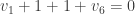
This simply tells us $v_1=v_6=v_7$ . By majority vote, we get $c = (1,1,1,1,1,1,1)$ .

Future coding theory in Sage projects

Posted on 2008/12/11 by wdjoyner

Here are a few ideas for future Sage projects in error-correcting codes.

Needed in Sage is

a rewrite in Cython, for speed,
special decoding algorithms, also in Cython,
for special decoders, it seems to me that one either needs

more classes (eg, a CyclicCodes class), each of which will have a decode method, or
another attribute, such as a name (string) which can be used to determine which decoder method to use.

codes over Rings (Cesar Agustin Garcia Vazquez is working on this)
codes defined from finite groups fings – for example split group codes,
a fast minimum distance function (followed by a fast weight distribution function), valid for all characteristics.

It seems more “Pythonic” to add more classes for decoders, but I am not sure.

Steiner systems and codes

Posted on 2008/10/02 by wdjoyner

A t-(v,k,λ)-design D=(P,B) is a pair consisting of a set P of points and a collection B of k-element subsets of P, called blocks, such that the number r of blocks that contain any point p in P is independent of p, and the number λ of blocks that contain any given t-element subset T of P is independent of the choice of T. The numbers v (the number of elements of P), b (the number of blocks), k, r, λ, and t are the parameters of the design. The parameters must satisfy several combinatorial identities, for example:

$\lambda _i = \lambda \left(\begin{array}{c} v-i\\ t-i\end{array}\right)/\left(\begin{array}{c} k-i\\ t-i\end{array}\right)$

where $\lambda _i$ is the number of blocks that contain any i-element set of points.

A Steiner system S(t,k,v) is a t-(v,k,λ) design with λ=1. There are no Steiner systems known with t>5. The ones known (to me anyway) for t=5 are as follows:

S(5,6,12), S(5,6,24), S(5,8,24), S(5,7,28), S(5,6,48), S(5,6,72), S(5,6,84),
S(5,6,108), S(5,6,132), S(5,6,168), and S(5,6,244).

Question: Are there others with t=5? ANy with $t>5$?

A couple of these are well-known to arise as the support of codewords of a constant weight in a linear code C (as in the Assmus-Mattson theorem, discussed in another post) in the case when C is a Golay code (S(5,6,12) and S(5,8,24)). See also the wikipedia entry for Steiner system.

Question: Do any of these others arise “naturally from coding theory” like these two do? I.e., do they all arise as the support of codewords of a constant weight in a linear code C via Assmus-Mattson?

Here is a Sage example to illustrate the case of S(5,8,24):

sage: C = ExtendedBinaryGolayCode()
sage: C.assmus_mattson_designs(5)
[‘weights from C: ‘,
[8, 12, 16, 24],
‘designs from C: ‘,
[[5, (24, 8, 1)], [5, (24, 12, 48)], [5, (24, 16, 78)], [5, (24, 24, 1)]],
‘weights from C*: ‘,
[8, 12, 16],
‘designs from C*: ‘,
[[5, (24, 8, 1)], [5, (24, 12, 48)], [5, (24, 16, 78)]]]
sage: C.assmus_mattson_designs(6)
0
sage: blocks = [c.support() for c in C if hamming_weight(c)==8]; len(blocks)
759

The Assmus-Mattson Theorem, Golay codes, and Mathieu groups

Posted on 2008/05/25 by wdjoyner

A block design is a pair $(X,B)$ , where $X$ is a non-empty finite set of $v>0$ elements called points, and $B$ is a non-empty finite multiset of size $b$ whose elements are called blocks, such that each block is a non-empty finite multiset of $k$ points. A design without repeated blocks is called a simple block design. If every subset of points of size $t$ is contained in exactly $\lambda$ blocks the the block design is called a $t$ — $(v,k,\lambda)$ design (or simply a $t$ -design when the parameters are not specfied). When $\lambda = 1$ then the block design is called a $S(t,k,v)$ Steiner system.

Let $C$ be an [ $n,k,d$ ] code and let $C_i = \{ c \in C\ |\ wt(c) = i\}$ denote the weight $i$ subset of codewords of weight $i$ . For each codeword $c\in C$ , let $supp(c)=\{i\ |\ c_i\not= 0\}$ denote the support of the codeword.

The first example below means that the binary [ $24,12,8$ ]-code $C$ has the property that the (support of the) codewords of weight 8 (resp, 12, 16) form a 5-design.

Example: Let $C$ denote the extended binary Golay code of length $24$ . This is a self-dual [ $24,12,8$ ]-code. The set $X_8 = \{supp(c)\ |\ c \in C_8\}$ is a $5-(24, 8, 1)$ design; $X_{12} = \{supp(c)\ |\ c \in C_{12}\}$ is a $5-(24, 12, 48)$ design;and, $X_{16} = \{supp(c)\ |\ c \in C_{16}\}$ is a $5-(24, 16, 78)$ design.

This is a consequence of the following theorem of Assmus and Mattson.

Assmus and Mattson Theorem (section 8.4, page 303 of [HP]):

Let $A_0, A_1, ..., A_n$ be the weight distribution of the codewords in a binary linear [ $n , k, d$ ] code $C$ , and let $A_0^\perp, A_1^\perp, ..., A_n^\perp$ be the weight distribution of the codewords in its dual [ $n,n-k, d^\perp$ ] code $C^\perp$ . Fix a $t$ , $0<t<d$ , and let $s = |\{ i\ |\ A_i^\perp \not= 0, 0<i\leq n-t\, \}|$ .
Assume $s\leq d-t$ .

If $A_i\not= 0$ and $d\leq i\leq n$ then $C_i = \{ c \in C\ |\ wt(c) = i\}$ holds a simple $t$ -design.
If $A_i^\perp\not= 0$ and $d^\perp\leq i\leq n-t$ then $C_i^\perp = \{ c \in C^\perp \ |\ wt(c) = i\}$ holds a simple $t$ –design.
If $A_i^\perp\not= 0$ and $d^\perp\leq i\leq n-t$ then $C_i^\perp = \{ c \in C^\perp \ |\ wt(c) = i\}$ holds a simple $t$ –design.

In the Assmus and Mattson Theorem, $X$ is the set $\{1,2,...,n\}$ of coordinate locations and $B = \{supp(c)\ |\ c \in C_i\}$ is the set of supports of the codewords of $C$ of weight $i$ . Therefore, the parameters of the $t$ -design for $C_i$ are

$t$ = given,
$v = n$ ,
$k = i$ , (this k is not to be confused with dim(C)!),
$b = A_i$ ,
$\lambda = b*binomial(k,t)/binomial(v,t)$

(by Theorem 8.1.6, p. 294, in \cite{HP}). Here is a SAGE example.

sage: C = ExtendedBinaryGolayCode() sage: C.assmus_mattson_designs(5) ['weights from C: ', [8, 12, 16, 24], 'designs from C: ', [[5, (24, 8, 1)], [5, (24, 12, 48)], [5, (24, 16, 78)], [5, (24, 24, 1)]], 'weights from C*: ', [8, 12, 16], 'designs from C*: ', [[5, (24, 8, 1)], [5, (24, 12, 48)], [5, (24, 16, 78)]]] sage: C.assmus_mattson_designs(6) 0

The automorphism group of the extended binary Golay code is the Mathieu group $M_{24}$ . Moreover, the code is spanned by the codewords of weight 8.

References:
[HP] W. C. Huffman, V. Pless, Fundamentals of error-correcting codes, Cambridge Univ. Press, 2003.
[CvL] P. Cameron, J. van Lint, Graphs, codes and designs, Cambridge Univ. Press, 1980.

Yet Another Mathblog

Tag Archives: coding theory

Searching with lies, 1

Lester Hill’s “The checking of the accuracy …”, part 7

Lester Hill’s “The checking of the accuracy …”, part 6

Lester Hill’s “The checking of the accuracy …”, part 5

Lester Hill’s “The checking of the accuracy …”, part 4

Remarks on the Hamming [7.4.3] code and Sage

Future coding theory in Sage projects

Steiner systems and codes

The Assmus-Mattson Theorem, Golay codes, and Mathieu groups