Caroline Melles and I have written a preprint that collects numerous examples of harmonic quotient morphisms 


I’ll post it to the math arxiv at some point but if you are interested now, here’s a copy: click here for pdf.
Caroline Melles and I have written a preprint that collects numerous examples of harmonic quotient morphisms
I’ll post it to the math arxiv at some point but if you are interested now, here’s a copy: click here for pdf.
The 1874 poem “The Mathematician in Love” by Scottish mechanical engineer William Rankine (in the book From Songs and Fables) has been published in many places (e.g., poetry.com, New Scientist and the scanned version is available at the internet archive. However, the mathematical equations Rankine presented at the end of his poem are only available in the scanned versions. As WordPress can render LaTeX, the poem quoted below includes those last few lines.
The Mathematician in Love
William J. M. Rankine
I.
A mathematician fell madly in love
With a lady, young, handsome, and charming:
By angles and ratios harmonic he strove
Her curves and proportions all faultless to prove,
As he scrawled hieroglyphics alarming.
II.
He measured with care, from the ends of a base.
The arcs which her features subtended:
Then he framed transcendental equations, to trace
The flowing outlines of her figure and face.
And thought the result very splendid.
III.
He studied (since music has charms for the fair)
The theory of fiddles and whistles, —
Then composed, by acoustic equations, an air,
Which, when ’twas performed, made the lady’s long hair
Stand on end, like a porcupine’s bristles.
IV.
The lady loved dancing: – he therefore applied.
To the polka and waltz, an equation;
But when to rotate on his axis he tried.
His centre of gravity swayed to one side.
And he fell, by the earth’s gravitation.
V.
No doubts of the fate of his suit made him pause.
For he proved, to his own satisfaction.
That the fair one returned his affection; – “because,
As every one knows, by mechanical laws,
Re-action is equal to action.”
VI.
“Let x denote beauty, – y manners well-bred, –
x, Fortune, – (this last is essential), –
Let L stand for love” – our philosopher said, –
“Then z is a function of x, y and 0,
Of the kind which is known as potential.”
VII.
“Now integrate L with respect to dt,
(t Standing for time and persuasion);
Then, between proper limits, ’tis easy to see,
The definite integral Marriage must be: —
(A very concise demonstration).”
VIII.
Said he – “If the wandering course of the moon
By Algebra can be predicted,
The female affections must yield to it soon” –
But the lady ran off with a dashing dragoon,
And left him amazed and afflicted.
End notes:
Equation referred to in Stanza VI.–
Equation referred to in Stanza VII.–
Here’s a shuffle I’ve not seen before:


In memory of the great German mathematician Edmund Landau (1877-1938, see also this bio), I call this the Landau shuffle. As with any card shuffle, this shuffle permutes the original ordering of the cards. To restore the deck to it’s original ordering you must perform this shuffle exactly 180180 times. (By the way, this is called the order of the shuffle.) Yes, one hundred eighty thousand, one hundred and eighty times. Moreover, no other shuffle than this Landau shuffle will require more repetitions to restore the deck. So, in some sense, the Landau shuffle is the shuffle that most effectively rearranges the cards.

Now suppose we have a deck of 


Question: What is the largest possible order of a shuffle of this deck (and how do you construct it)?
This requires a tiny bit of group theory. You only need to know that any permutation of 


The Landau function 
Example: If 


Oddly, my favorite mathematical software program SageMath does not have an implementation of the Landau function, so we end with some SageMath code.
def landau_function(n):
    L = Partitions(n).list()
    lcms = [lcm(P) for P in L]
    return max(lcms)
Here is an example (the time is included to show this took about 2 seconds on my rather old mac laptop):
sage: time landau_function(52)
CPU times: user 1.91 s, sys: 56.1 ms, total: 1.97 s
Wall time: 1.97 s
180180
This was once posted on my USNA webpage. Since I’ve retired, I’m going to repost it here.
Coding Theory and Cryptography:
From Enigma and Geheimschreiber to Quantum Theory
(David Joyner, ed.) Springer-Verlag, 2000.
ISBN 3-540-66336-3
Summary: These are the proceedings of the “Cryptoday” Conference on Coding Theory, Cryptography, and Number Theory held at the U. S. Naval Academy during October 25-26, 1998. This book concerns elementary and advanced aspects of coding theory and cryptography. The coding theory contributions deal mostly with algebraic coding theory. Some of these papers are expository, whereas others are the result of original research. The emphasis is on geometric Goppa codes, but there is also a paper on codes arising from combinatorial constructions. There are both, historical and mathematical papers on cryptography.
Several of the contributions on cryptography describe the work done by the British and their allies during World War II to crack the German and Japanese ciphers. Some mathematical aspects of the Enigma rotor machine and more recent research on quantum cryptography are described. Moreover, there are two papers concerned with the RSA cryptosystem and related number-theoretic issues.
Chapters
For more cryptologic history, see the National Cryptologic Museum.
This is now out of print and will not be reprinted (as far as I know). The above pdf files are posted by written permission. I thank Springer-Verlag for this.
At first, you might think this is obvious – just “clip” off each corner of the tetrahedron 

First, color the vertices of the tetrahedron in some way.

The coloring below corresponds to a harmonic morphism 
All others are obtained from this by permuting the colors. They are all covers of 

In an earlier post titled Mathematical romantic? I mentioned some papers I inherited of one of my mathematical hero’s Andre Weil with his signature. In fact, I was fortunate enough to go to dinner with him once in Princeton in the mid-to-late 1980s – a very gentle, charming person with a deep love of mathematics. I remember he said he missed his wife, Eveline, who passed away in 1986. (They were married in 1937.)
All this is simply to motivate the question, why did I get these papers? First, as mentioned in the post, I was given Larry Goldstein‘s old office and he either was kind enough to gift me his old preprints or left them to be thrown away by the next inhabitant of his office. BTW, if you haven’t heard of him, Larry was a student of Shimura, when became a Gibbs Fellow at Yale, then went to the University of Maryland at COllege Park in 1969. He wrote lots of papers (and books) on number theory, eventually becoming a full professor, but eventually settled into computers and data science work. He left the University of Maryland about the time I arrived in the early 1980s to create some computer companies that he ran.
This motivates the question: How did Larry get these papers of Weil? I think Larry inherited them from Mountjoy (who died before Larry arrived at UMCP, but more on him later). This motivates the question, who is Mountjoy and how did he get them?
I’ve done some digging around the internet and here’s what I discovered.
The earliest mention I could find is when he was listed as a recipient of an NSF Fellowship in “Annual Report of the National Science Foundation: 1950-1953” under Chicago, Illinois, Mathematics, 1953. So he was a grad student at the University of Chicago in 1953. Andre Weil was there at the time. (He left sometime in 1958.) Mountjoy could have gotten the notes of Andre Weil then. Just before Weil left Chicago, Walter Lewis Baily arrived (in 1957, to be exact). This is important because in May 1965 the Notices of the AMS reported that reported:
Mountjoy, Robert Harbison
Abelian varieties attached to representations of discontinuous groups (S. Mac Lane and W. L. Baily)
(His thesis was published posthumously in American Journal of Mathematics Vol. 89 (1967)149-224.) This thesis is in a field studied by Weil and Baily but not Saunders.
But we’re getting ahead of ourselves. The 1962 issue of Maryland Magazine had this:
Mathematics Grant
A team of University of Maryland mathematics researchers have received a grant of $53,000 from the National Science Foundation to continue some technical investigations they started two years ago.
The mathematical study they are directing is entitled “Problems in Geometric Function Theory.” The project is under the direction of Dr. James Hummel. Dr. Mischael Zedek. and Prof. Robert H. Mountjoy, all of the Mathematics Department. They are assisted by four graduate-student researchists. The $53,000 grant is a renewal of an original grant which was made two years ago.
We know he was working at UMCP in 1962.
Here’s the sad news.
The newspaper Democrat and Chronicle, from Rochester, New York, on Wednesday, May 25, 1965 (Page 40) published the news that Robert H. Mountjoy “Died suddenly at Purcellville, VA, May 23, 1965”. I couldn’t read the rest (it’s behind a paywall but I could see that much). The next day, they published more: “Robert H. Mountjoy, son-in-law of Mr and Mrs Allen P Mills of Brighton, was killed in a traffic crash in Virgina. Mountjoy, about 30, a mathematics instructors at the University of Maryland, leaves a widow Sarah Mills Mountjoy and a 5-month old son Alexander, and his parents Mr and Mrs Lucius Mountjoy of Chicago.”
It’s so sad. The saying goes “May his memory be a blessing.” I never met him, but from what I’ve learned of Mountjoy, his memory is indeed a blessing.
A little over 10 years ago, M. Baker and S. Norine (I’ve also seen this name spelled Norin) wrote a terrific paper on harmonic morphisms between simple, connected graphs (see “Harmonic morphisms and hyperelliptic graphs” – you can find a downloadable pdf on the internet of you google for it). Roughly speaking, a harmonic function on a graph is a function in the kernel of the graph Laplacian. A harmonic morphism between graphs is, roughly speaking, a map from one graph to another that preserves harmonic functions.
They proved quite a few interesting results but one of the most interesting, I think, is their graph-theoretic analog of the Riemann-Hurwitz formula. We define the genus of a simple connected graph 
It represents the minimum number of edges that must be removed from the graph to make it into a tree (so, a tree has genus 0).
Riemann-Hurwitz formula (Baker and Norine): Let 


I’m not going to define them here but 

I simply want to record a very easy corollary to this, assuming 

Corollary: Let 
to a connected
Then
This page is modeled after the handy wikipedia page Table of simple cubic graphs of “small” connected 3-regular graphs, where by small I mean at most 11 vertices.
These graphs are obtained using the SageMath command graphs(n, [4]*n), where n = 5,6,7,… .
5 vertices: Let 
4reg5a: The only such 4-regular graph is the complete graph 

We have
 .)
.)
6 vertices: Let 
4reg6a: The first (and only) such 4-regular graph is the graph 


We have
7 vertices: Let 
4reg7a: The 1st such 4-regular graph is the graph 

We have
4reg7b: The 2nd such 4-regular graph is the graph 
We have
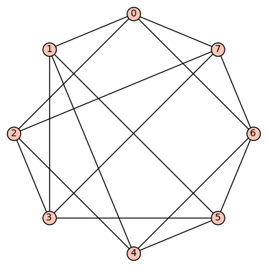
8 vertices: Let 
4reg8a: The 1st such 4-regular graph is the graph 
We have
 and
and  .
.4reg8b: The 2nd such 4-regular graph is the graph
We have
 ,
,  ,
,  ,
,  .
.4reg8c: The 3rd such 4-regular graph is the graph 
We have
 and is generated by (5,6), (4,7), (3,4), (2,5), (1,2), (0,1)(2,3)(4,5)(6,7).
4reg8d: The 4th such 4-regular graph is the graph 

We have
4reg8e: The 5th such 4-regular graph is the graph 
We have
4reg8f: The 6th (and last) such 4-regular graph is the bipartite graph 


We have
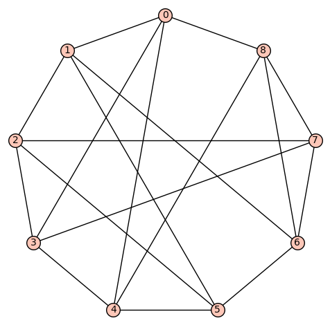
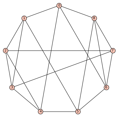
9 vertices: Let 
Without going into details, it is possible to theoretically prove that there are no harmonic morphisms from any of these graphs to either the cycle graph 


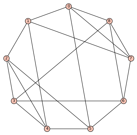
d4reg9-1
Gamma edges: E1 = [(0, 1), (0, 2), (0, 7), (0, 8), (1, 2), (1, 3), (1, 7), (2, 3), (2, 8), (3, 4), (3, 5), (4, 5), (4, 6), (4, 8), (5, 6), (5, 7), (6, 7), (6, 8)]
diameter:  2
girth:  3
is connected:  True
aut gp size:  12
aut gp gens:  [(1,2)(4,5)(7,8), (0,1)(3,8)(5,6), (0,4)(1,5)(2,6)(3,7)]

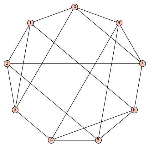
d4reg9-2
Gamma edges: E1 = [(0, 1), (0, 3), (0, 7), (0, 8), (1, 2), (1, 3), (1, 7), (2, 3), (2, 5), (2, 8), (3, 4), (4, 5), (4, 6), (4, 8), (5, 6), (5, 7), (6, 7), (6, 8)]
diameter:  2
girth:  3
is connected:  True
aut gp size:  2
aut gp gens:  [(0,5)(1,6)(2,8)(3,4)]

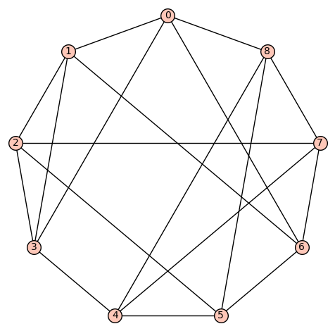
d4reg9-3
Gamma edges: E1 = [(0, 1), (0, 2), (0, 7), (0, 8), (1, 2), (1, 3), (1, 4), (2, 3), (2, 8), (3, 4), (3, 5), (4, 5), (4, 6), (5, 6), (5, 7), (6, 7), (6, 8), (7, 8)]
diameter:  2
girth:  3
is connected:  True
aut gp size:  18
aut gp gens:  [(1,7)(2,8)(3,6)(4,5), (0,1,4,6,8,2,3,5,7)]

d4reg9-4
Gamma edges: E1 = [(0, 1), (0, 5), (0, 7), (0, 8), (1, 2), (1, 4), (1, 7), (2, 3), (2, 4), (2, 5), (3, 4), (3, 6), (3, 8), (4, 5), (5, 6), (6, 7), (6, 8), (7, 8)]
diameter:  2
girth:  3
is connected:  True
aut gp size:  4
aut gp gens:  [(2,4), (0,6)(1,3)(7,8)]
d4reg9-5
Gamma edges: E1 = [(0, 1), (0, 3), (0, 5), (0, 8), (1, 2), (1, 4), (1, 7), (2, 3), (2, 5), (2, 7), (3, 4), (3, 8), (4, 5), (4, 6), (5, 6), (6, 7), (6, 8), (7, 8)]
diameter:  2
girth:  3
is connected:  True
aut gp size:  12
aut gp gens:  [(1,5)(2,4)(6,7), (0,1)(2,3)(4,5)(7,8)]

d4reg9-6
Gamma edges: E1 = [(0, 1), (0, 3), (0, 7), (0, 8), (1, 2), (1, 5), (1, 6), (2, 3), (2, 5), (2, 6), (3, 4), (3, 8), (4, 5), (4, 7), (4, 8), (5, 6), (6, 7), (7, 8)]
diameter:  2
girth:  3
is connected:  True
aut gp size:  8
aut gp gens:  [(2,6)(3,7), (0,3)(1,2)(4,7)(5,6)]

d4reg9-7
Gamma edges: E1 = [(0, 1), (0, 3), (0, 4), (0, 8), (1, 2), (1, 3), (1, 6), (2, 3), (2, 5), (2, 7), (3, 4), (4, 5), (4, 8), (5, 6), (5, 7), (6, 7), (6, 8), (7, 8)]
diameter:  2
girth:  3
is connected:  True
aut gp size:  2
aut gp gens:  [(0,3)(1,4)(2,8)(5,6)]

d4reg9-8
Gamma edges: E1 = [(0, 1), (0, 3), (0, 7), (0, 8), (1, 2), (1, 3), (1, 6), (2, 3), (2, 5), (2, 7), (3, 4), (4, 5), (4, 6), (4, 8), (5, 6), (5, 8), (6, 7), (7, 8)]
diameter:  2
girth:  3
is connected:  True
aut gp size:  2
aut gp gens:  [(0,8)(1,5)(2,6)(3,4)]
d4reg9-9
Gamma edges: E1 = [(0, 1), (0, 3), (0, 6), (0, 8), (1, 2), (1, 3), (1, 6), (2, 3), (2, 5), (2, 7), (3, 4), (4, 5), (4, 7), (4, 8), (5, 6), (5, 8), (6, 7), (7, 8)]
diameter:  2
girth:  3
is connected:  True
aut gp size:  4
aut gp gens:  [(5,7), (0,3)(2,6)(4,8)]
d4reg9-10
Gamma edges: E1 = [(0, 1), (0, 3), (0, 5), (0, 8), (1, 2), (1, 4), (1, 6), (2, 3), (2, 5), (2, 7), (3, 4), (3, 7), (4, 5), (4, 8), (5, 6), (6, 7), (6, 8), (7, 8)]
diameter:  2
girth:  3
is connected:  True
aut gp size:  16
aut gp gens:  [(2,6)(3,8), (1,5), (0,1)(2,3)(4,5)(6,8)]

d4reg9-11
Gamma edges: E1 = [(0, 1), (0, 3), (0, 7), (0, 8), (1, 2), (1, 4), (1, 6), (2, 3), (2, 5), (2, 7), (3, 4), (3, 5), (4, 5), (4, 8), (5, 6), (6, 7), (6, 8), (7, 8)]
diameter:  2
girth:  3
is connected:  True
aut gp size:  8
aut gp gens:  [(2,4)(7,8), (0,2)(3,7)(4,6)(5,8)]

d4reg9-12
Gamma edges: E1 = [(0, 1), (0, 3), (0, 6), (0, 8), (1, 2), (1, 4), (1, 6), (2, 3), (2, 5), (2, 7), (3, 4), (3, 7), (4, 5), (4, 8), (5, 6), (5, 8), (6, 7), (7, 8)]
diameter:  2
girth:  3
is connected:  True
aut gp size:  18
aut gp gens:  [(1,6)(2,5)(3,8)(4,7), (0,1,6)(2,7,3)(4,5,8), (0,2)(1,3)(5,8(6,7)]

d4reg9-13
Gamma edges: E1 = [(0, 1), (0, 3), (0, 4), (0, 8), (1, 2), (1, 5), (1, 6), (2, 3), (2, 5), (2, 7), (3, 4), (3, 7), (4, 5), (4, 8), (5, 6), (6, 7), (6, 8), (7, 8)]
diameter:  2
girth:  3
is connected:  True
aut gp size:  8
aut gp gens:  [(2,6)(3,8), (0,1)(2,3)(4,5)(6,8), (0,4)(1,5)]
d4reg9-14
Gamma edges: E1 = [(0, 1), (0, 3), (0, 4), (0, 8), (1, 2), (1, 5), (1, 8), (2, 3), (2, 5), (2, 7), (3, 4), (3, 7), (4, 5), (4, 6), (5, 6), (6, 7), (6, 8), (7, 8)]
diameter:  2
girth:  3
is connected:  True
aut gp size:  72
aut gp gens:  [(2,5)(3,4)(6,7), (1,3)(4,8)(5,7), (0,1)(2,3)(4,5)]

d4reg9-15
Gamma edges: E1 = [(0, 1), (0, 4), (0, 6), (0, 8), (1, 2), (1, 3), (1, 5), (2, 3), (2, 4), (2, 7), (3, 4), (3, 7), (4, 5), (5, 6), (5, 8), (6, 7), (6, 8), (7, 8)]
diameter:  2
girth:  3
is connected:  True
aut gp size:  32
aut gp gens:  [(6,8), (2,3), (1,4), (0,1)(2,6)(3,8)(4,5)]
d4reg9-16
Gamma edges: E1 = [(0, 1), (0, 3), (0, 7), (0, 8), (1, 2), (1, 4), (1, 5), (2, 3), (2, 4), (2, 5), (3, 7), (3, 8), (4, 5), (4, 6), (5, 6), (6, 7), (6, 8), (7, 8)]
diameter:  2
girth:  3
is connected:  True
aut gp size:  16
aut gp gens:  [(7,8), (4,5), (0,1)(2,3)(4,7)(5,8), (0,2)(1,3)(4,7)(5,8)]

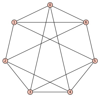
10 vertices: Let 
Example 1: The quartic, symmetric graph on 10 vertices that is not distance regular is depicted below. It has diameter 2, girth 4, chromatic number 3, and has an automorphism group of order 320 generated by 
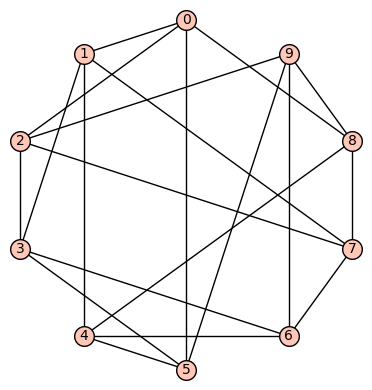
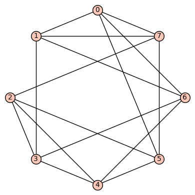
Example 2: The quartic, distance regular, symmetric graph on 10 vertices is depicted below. It has diameter 3, girth 4, chromatic number 2, and has an automorphism group of order 240 generated by 

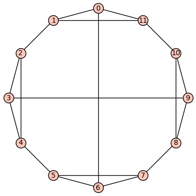
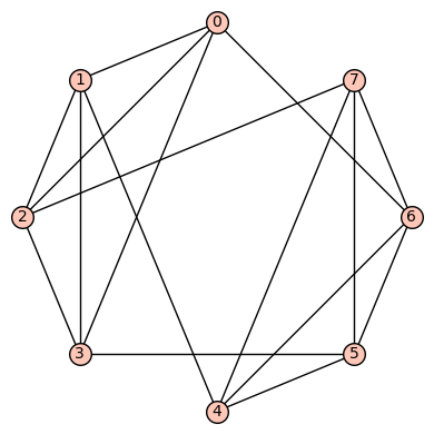
11 vertices: There are (up to isomorphism) exactly 265 4-regular connected graphs on 11 vertices. Only two of these are vertex transitive. None are distance regular or edge transitive.
Example 1: One of the vertex transitive graphs is depicted below. It has diameter 2, girth 4, chromatic number 3, and has an automorphism group of order 22 generated by 


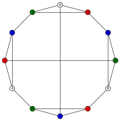
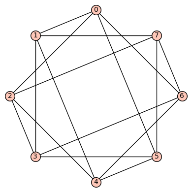
Example 2:The second vertex transitive graph is depicted below. It has diameter 3, girth 3, chromatic number 4, and has an automorphism group of order 22 generated by 


I recently learned about a new class of seemingly complicated, but in fact very simple functions which are called by several names, but perhaps most commonly as NCF Boolean functions (NCF is an abbreviation for “nested canalyzing function,” a term used by mathematical biologists). These functions were independently introduced by theoretical computer scientists in the 1960s using the term unate cascade functions. As described in [JRL2007] and [LAMAL2013], these functions have applications in a variety of scientific fields. This post describes these functions.
A Boolean function of n variables is simply a function 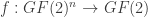


denote the restriction map sending 
will be called coordinate hyperplanes (


If 


For details, see for example Li and Adeyeye [LA2012].
REFERENCES
[JRL2007] A.S. Jarrah, B. Raposa, R. Laubenbachera, “Nested Canalyzing, Unate Cascade, and Polynomial Functions,” Physica D. 2007 Sep 15; 233(2): 167–174.
[LA2012] Y. Li, J.O. Adeyeye, “Sensitivity and block sensitivity of nested canalyzing function,” ArXiV 2012 preprint. (A version of this paper was published later in Theoretical Comp. Sci.)
[LAMAL2013] Y. Li, J.O. Adeyeye, D. Murrugarra, B. Aguilar, R. Laubenbacher, “Boolean nested canalizing functions: a comprehensive analysis,” ArXiV, 2013 preprint.
The files below were on my teaching page when I was a college teacher. Since I retired, they disappeared. Samuel Lelièvre found an archived copy on the web, so I’m posting them here.
The files are licensed under the Attribution-ShareAlike Creative Commons license.
Course review: pdf
Love, War, and Zombies, pdf
This set of slides is of a lecture I would give if there was enough time towards the end of the semester


![{\rm genus}(\Gamma_2)-1 = {\rm deg}(\phi)({\rm genus}(\Gamma_1)-1)+\sum_{x\in V_2} [m_\phi(x)+\frac{1}{2}\nu_\phi(x)-1].](https://s0.wp.com/latex.php?latex=%7B%5Crm+genus%7D%28%5CGamma_2%29-1+%3D+%7B%5Crm+deg%7D%28%5Cphi%29%28%7B%5Crm+genus%7D%28%5CGamma_1%29-1%29%2B%5Csum_%7Bx%5Cin+V_2%7D+%5Bm_%5Cphi%28x%29%2B%5Cfrac%7B1%7D%7B2%7D%5Cnu_%5Cphi%28x%29-1%5D.&bg=ffffff&fg=323232&s=0&c=20201002)


You must be logged in to post a comment.