This post summarizes some joint research with Charles Celerier, Caroline Melles, and David Phillips.
Let  be a Boolean function. (We identify
  with either the real numbers
  or the binary field
  . Hopefully, the context makes it clear which one is used.)
Define a partial order  on
on  as follows: for each
  , we say
  whenever we have
  ,
,  , …,
, …,  . A Boolean function is called monotone (increasing) if whenever we have then we also have
  .
.
Note that if  and
and  are monotone then (a)
  is also monotone, and (b)
  . (Overline means bit-wise complement.)
Definition:
Let be any monotone function. We say that  is the least support of if
  consists of all vectors in
  which are smallest in the partial ordering
  on . We say a subset
  of is admissible if for all
  ,
,  and
and 
Monotone functions on are in a natural one-to-one correspondence with the collection of admissible sets.
Example:
Here is an example of a monotone function whose least support vectors are given by

illustrated in the figure below.

The algebraic normal form is  .
.
The following result is due to Charles Celerier.
Theorem:
Let be a monotone function whose least support vectors are given by  . Then

The following example is due to Caroline Melles.
Example:
Let be the monotone function whose least support is

Using the Theorem above, we obtain the compact algebraic form

This function is monotone yet has no vanishing Walsh-Hadamard transform values. To see this, we attach the file afsr.sage available from Celerier (https://github.com/celerier/oslo/), then run the following commands.
sage: V = GF(2)^(6)
sage: L = [V([1,1,0,0,1,1]),V([0,0,1,1,1,1]), V([1,1,1,1,0,0])]
sage: f = monotone_from_support(L)
sage: is_monotone(f)
True
These commands simply construct a Boolean function whose least support are the vectors in L. Next, we compute the Walsh-Hadamard transform of this using both the method built into Sage’s sage.crypto module, and the function in afsr.sage.
sage: f.walsh_hadamard_transform()
(-44, -12, -12, 12, -12, 4, 4, -4, -12, 4, 4, -4, 12, -4, -4, 4, -12, 4, 4, -4, 4, 4, 4, -4, 4, 4, 4, -4, -4,
 -4, -4, 4, -12, 4, 4, -4, 4, 4, 4, -4, 4, 4, 4, -4, -4, -4, -4, 4, 12, -4, -4, 4, -4, -4, -4, 4, -4, -4, -4, 4, 4, 4, 4, -4)
sage: f.algebraic_normal_form()
x0*x1*x2*x3 + x0*x1*x4*x5 + x2*x3*x4*x5
sage: x0,x1,x2,x3,x4,x5 = var("x0,x1,x2,x3,x4,x5")
sage: g = x0*x1*x2*x3 + x0*x1*x4*x5 + x2*x3*x4*x5
sage: Omega = [v for v in V if g(x0=v[0], x1=v[1], x2=v[2], x3=v[3],
     x4=v[4], x5=v[5])0]
sage: len(Omega)
10
sage: g = lambda x: x[0]*x[1]*x[2]*x[3] + x[0]*x[1]*x[4]*x[5] + x[2]*x[3]*x[4]*x[5]
sage: [walsh_transform(g,a) for a in V]
[44, 12, 12, -12, 12, -4, -4, 4, 12, -4, -4, 4, -12, 4, 4, -4, 12, -4, -4, 4, -4, -4, -4, 4, -4, -4, -4, 4, 4,
 4, 4, -4, 12, -4, -4, 4, -4, -4, -4, 4, -4, -4, -4, 4, 4, 4, 4, -4, -12, 4, 4, -4, 4, 4, 4, -4, 4, 4, 4, -4, -4, -4, -4, 4]
(Note: the Walsh transform method in the BooleanFunction class in Sage differs by a sign from the standard definition.) This verifies that there are no values of the Walsh-Hadamard transform which are  .
.
More details can be found in the paper listed here. I end with two questions (which I think should be answered “no”).
Question: Are there any monotone functions of  variables having no free variables of degree
  ?
?
Question: Are there any monotone functions of most than two variables which are bent?

![{\mathbb{Z}}[V]](https://s0.wp.com/latex.php?latex=%7B%5Cmathbb%7BZ%7D%7D%5BV%5D&bg=ffffff&fg=323232&s=0&c=20201002)


![[D]](https://s0.wp.com/latex.php?latex=%5BD%5D&bg=ffffff&fg=323232&s=0&c=20201002)


 be a prime power such that
  . Note that this implies that the unique finite field of order
  , has a square root of
  . Now let
  and
and
 if and only if
  . By definition
  is the
  (with multiplicity
  ) and
) and (both with multiplicity
  , where
  is prime, then
  has order
  .
. ” above; I was having trouble rendering it in html.) Below is an example.
 , it has only three distinct eigenvalues, and its automorphism group is order
  .
. :
: :
:

 and
and  are matrices of the same size. Then
  .
.
 , if k <= n/2 and
  , if
, if  Let
Let  , where
  and
and  is the symmetric group of order
 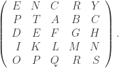 BTW, the
  analog is:
  .
. case is in Alasdair’s book):
 then this is a
  -time algorithm. For comparison, the
  , which is
  -time algorithm for “dense” graphs. Except for “sparse” graphs, Floyd-Warshall-Roy is better than an interated implementation of Bellman-Ford.
You must be logged in to post a comment.