This is a very short introductory survey of graph-theoretic properties of Boolean functions.
I don’t know who first studied Boolean functions for their own sake. However, the study of Boolean functions from the graph-theoretic perspective originated in Anna Bernasconi‘s thesis. More detailed presentation of the material can be found in various places. For example, Bernasconi’s thesis (e.g., see [BC]), the nice paper by P. Stanica (e.g., see [S], or his book with T. Cusick), or even my paper with Celerier, Melles and Phillips (e.g., see [CJMP], from which much of this material is literally copied).
For a given positive integer 
with its support

For each 


where 


denote the cardinality of the support. We call a Boolean function even (resp., odd) if 


be the binary representation ordered with least significant bit last (so that, for example, 
Let 

The Walsh-Hadamard transform of 


where we define 

for 
Example
A Boolean function of three variables cannot be bent. Let
This is simply the function 
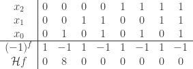

Here is some Sage code verifying this:
sage: from sage.crypto.boolean_function import *
sage: f = BooleanFunction([0,1,0,1,0,1,0,1])
sage: f.algebraic_normal_form()
x0
sage: f.walsh_hadamard_transform()
(0, -8, 0, 0, 0, 0, 0, 0)
(The Sage method walsh_hadamard_transform is off by a sign from the definition we gave.) We will return to this example later.
Let 
We shall assume throughout and without further mention that 


For each vertex 


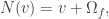
where 


Example:
Returning to the previous example, we construct its Cayley graph.
First, attach afsr.sage from [C] in your Sage session.
     sage: flist = [0,1,0,1,0,1,0,1]
     sage: V = GF(2)ˆ3
     sage: Vlist = V.list()
     sage: f = lambda x: GF(2)(flist[Vlist.index(x)])
     sage: X = boolean_cayley_graph(f, 3)
     sage: X.adjacency_matrix()
     [0 1 0 1 0 1 0 1]
     [1 0 1 0 1 0 1 0]
     [0 1 0 1 0 1 0 1]
     [1 0 1 0 1 0 1 0]
     [0 1 0 1 0 1 0 1]
     [1 0 1 0 1 0 1 0]
     [0 1 0 1 0 1 0 1]
     [1 0 1 0 1 0 1 0]
     sage: X.spectrum()
     [4, 0, 0, 0, 0, 0, 0, -4]
     sage: X.show(layout="circular")

In her thesis, Bernasconi found a relationship between the spectrum of the Cayley graph

(the eigenvalues 


between the spectrum of the Cayley graph
References:
[BC] A. Bernasconi and B. Codenotti, Spectral analysis of Boolean functions as a graph eigenvalue problem, IEEE Trans. Computers 48(1999)345-351.
[CJMP] Charles Celerier, David Joyner, Caroline Melles, David Phillips, On the Hadamard transform of monotone Boolean functions, Tbilisi Mathematical Journal, Volume 5, Issue 2 (2012), 19-35.
[S] P. Stanica, Graph eigenvalues and Walsh spectrum of Boolean functions, Integers 7(2007)\# A32, 12 pages.
Here’s an excellent video of Pante Stanica on interesting applications of Boolean functions to cryptography (30 minutes):
 be a Boolean function. (We identify
  with either the real numbers
  or the binary field
  . Hopefully, the context makes it clear which one is used.)
 on
on  , we say
  whenever we have
  ,
,  , …,
, …,  . A Boolean function is called monotone (increasing) if whenever we have
  .
.  are monotone then (a)
  is also monotone, and (b)
  . (Overline means bit-wise complement.)
 is the least support of
  consists of all vectors in
  which are smallest in the partial ordering
  on
on  ,
,  and
and 


 .
. . Then


 .
. ?
?
You must be logged in to post a comment.