Lester Hill’s “The checking of the accuracy …”, part 9

We may inquire into the possibility of undisclosed errors occurring in the transmittal of the sequence:

\begin{array}{ccccccccccccccc}  f_1 & f_2 & f_3 & f_4 & f_5 & f_6 & f_7 & f_8 & f_9  & f_{10} & f_{11} & f_{12} & c_1 & c_2 & c_3 \\  5 & 17 & 13 & 21 & 0 & 8 & 6 & 0 & 11 & 0 & 11 & 11 & 6 & 15 & 2 \\  X & T & Y & P & V & Z & R & V & H & V & H & H & R & I & F \\  \end{array}

Invoking the theorem established in sections 4 and 5, and formulated at the close of section 5, we may assert:

  • (1) If not more than three errors are made in transmitting the fifteen letters of the sequence, and if the errors made affect the f_i only, the c_j being correctly transmitted, then the presence of error is certain to be disclosed.
  • (2) If not more than three errors are made, all told, but at least three of them affect the f_i, then the presence of error will enjoy only a

    1-{\rm in}-22^3\ \ \ \ \ (1-{\rm in}-10648)
    chance of escaping disclosure.

These assertions result at once from the theorem referred to. But a closer study of the reference matrix employed in this example permits us to replace them by the following more satisfactory statements:

  • (1′)
    If errors occur in not more than three of the fifteen elements of the sequence f_1f_2\dots f_{12}c_1 c_2 c_3, and if at least one of the particular elements f_{11}f_{12}c_2 is correctly transmitted, the presence of error will certainly be disclosed. But if exactly three errors are made, affecting presicely the elements f_{11}f_{12}c_2, the presence of error will enjoy a 1-in-22^2 (1-in-484) chance of escaping disclosure.
  • (2′)
    If more than three errors are made, then whatever the distribution of errors among the fifteen elements of the sequence, the presence of error will enjoy only a
    1-in-22^3 (1-in-10648) chance of escaping disclosure.

Assertions of this kind will be carefully established below, when a more important finite field is under consideration. The argument then made will be applicable in the case of any finite field. But it is worthwhile here to look more carefully into the exceptional distribution of errors which is italicized in (1′). This will help us note any weakness that ought to be avoided in the construction of reference matrices.

Suppose that exactly three errors are made, affecting precisely f_{11}f_{12}c_2. If the mutilated message is to check up, and the errors to escape disclosure, we must have (for error notations, see sections 4,5):

11\epsilon_{11}+12\epsilon_{12}=0,\ \ \   11^2\epsilon_{11}+12^2\epsilon_{12}=\delta_2,\ \ \   11^3\epsilon_{11}+12^3\epsilon_{12}=0.
These equations may be written:

11\epsilon_{11}+12\epsilon_{12}=0,\ \ \   6\epsilon_{11}+6\epsilon_{12}=\delta_2,\ \ \   20\epsilon_{11}+3\epsilon_{12}=0.
But 11\epsilon_{11}=-12\epsilon_{12} can be written 11\epsilon_{11}=11\epsilon_{12}, or \epsilon_{11}=\epsilon_{12}.
Etc. In this way, we find that the errors can escape disclosure if and only if

\epsilon_{11}=\epsilon_{12},\ \ \ {\rm and}\ \ \ \delta_{2}=12\epsilon_{11}.
The error \epsilon_{11} can be made quite arbitrarily. But then the values of \epsilon_{12} and \delta_2 are then completely determined. There is evidently a 1-in-484 chance – and no more – that the errors will fall out just right.

The trouble arises from the vanishing, in our reference matrix, of the two-rowed
determinant

\big{|}   \begin{array}{cc}  11 & 12 \\  11^3 & 12^3  \end{array}  \big{|} .
Note that

\big{|}   \begin{array}{cc}  11 & 12 \\  11^3 & 12^3  \end{array}  \big{|}   = 11\cdot 12\cdot  \big{|}   \begin{array}{cc}  1 & 1 \\  11^2 & 12^2  \end{array}  \big{|}   = 17 \big{|}   \begin{array}{cc}  1 & 1 \\  11^2 & 12^2  \end{array}  \big{|} =0,
since 11^2=12^2.

From the fact that \big{|}   \begin{array}{cc}  11 & 12 \\  11^3 & 12^3  \end{array}  \big{|} is the only vanishing determinant of any order in the matrix employed, all other assertions made in (1′) and (2′) are readily justified. This will be made clear in the following sections.

It will be advantageous, as shown more completely in subsequent sections, to employ reference matrices which contain the smallest possible number of vanishing determinants of any orders.

Lester Hill’s “The checking of the accuracy …”, part 8

Introductory example of checking

We may use the field F_{23} as the basis for a simple illustrative exercise in the actual procedure of checking. The general of the operations involved will thus be made clear, so far as modus operandi is concerned, and we shall be enabled to discuss more easily the pertinent mathematical details.

It is easy to set up telegraphic codes of high capacity using combinations of four letters each which are not required to be pronounceable. In fact, a sufficiently high capacity may be obtained when only
twenty-three letters of the alphabet are used at all. Hence we can omit any three letters whose Morse equivalents (dot-dash) are most frequently used. Let us suppose that we have before us a code of this kind which employs the letters

A\ \ B\ \ C\ \ E\ \ F\ \ G\ \ H\ \ I\ \ J\ \ L\ \ M\ \ N\ \ P\ \ Q\ \ R\ \ S\ \ T\ \ U\ \ V\ \ W\ \ X\ \ Y\ \ Z
and avoids, for reasons stated of for some good reason, the three letters

D\ \ K\ \ O\, .

Suppose that, by prearrangement with telegraphic correspondents, the letters used are paired in
an arbitrary, but fixed, way with the thwenty-three elements of F_{23}.
Let the pairings be, for instance:

\begin{tabular}{ccccccccccccccccccccccc}  A & B  & C & E & F & G & H  & I    & J    & L & M & N  & P   & Q   & R    & S & T   & U   & V & W & X   & Y & Z \\ \hline  4 & 7 & 9 & 14& 2 & 1 & 11 & 15 & 10 & 3 & 19 & 18 & 21 & 16 & 6 & 20 & 17 & 12 & 0 & 22 & 5 & 13 & 8 \\  \end{tabular}
or, in numerical arrangement:

\begin{tabular}{ccccccccccccccccccccccc}  0 & 1  & 2 & 3 & 4 & 5 & 6  & 7  & 8  & 9 & 10 & 11 & 12 & 13 & 14  & 15 & 16  & 17  & 18 & 19 & 20  & 21 & 22 \\ \hline  V & G & F & L& A & X & R & B & Z & C & J & H & U & Y & E & I & Q & T & N & M & S & P & W \\  \end{tabular}

A four-letter group (code word), such as EZRA or XTYP, will indicate a definite entry of a specific page of a definite code volume, several such volumes being perhaps employed in the code. An entry will, in general, be a phrase of sentence, or a group of phrases or sentences, commonly occurring in the class of messages for which the code has been constructed.

Suppose that we have agreed to provide, in our messages, three-letter checks upon groups of twelve letters; in other words, to check in one operation a sequence of three four-letter code words. The twelve letters of the three code words are thus expanded to fifteen; but we send just three telegraphic words — three combinations of five letters, each of which is, in general, unpronounceable.

For illustration, let the first three code words of a message be:

XTYP\ \ \ \ VZRV\ \ \ \ HVHH
The corresponding sequence of paired elements in F_{23} is:

5 \ \ 17\ \ 13\ \ 21\ \ 0\ \ 8\ \ 6\ \ 0\ \ 11\ \ 0\ \ 11\ \ 11.
This is our operand sequence f_i:

f_1 = 5,\ \ f_2=17,\ \ f_3=13,\ \ f_4=21,\ \ f_5=0,\ \dots,\ ,f_{12}=11.

Let us determine the checking matrix c_1, c_2, c_3 by using as reference matrix

\left(  \begin{array}{cccccccccccc}  1 & 2 & 3 & 4 & 5 & 6 & 7 & 8 & 9 & 10 & 11 & 12\\  1^2 & 2^2 & 3^2 & 4^2 & 5^2 & 6^2 & 7^2 & 8^2 & 9^2 & 10^2 & 11^2 & 12^2 \\  1^3 & 2^3 & 3^3 & 4^3 & 5^3 & 6^3 & 7^3 & 8^3 & 9^3 & 10^3 & 11^3 & 12^3 \\  \end{array}  \right)
Thus the c_j are to be

c_j = \sum_{i=1}^{12} i^jf_i\ \ \ \ (j = 1,2,3),

or

c_1 = \sum_{i=1}^{12} if_i.\ \ \ c_2 = \sum_{i=1}^{12} i^2f_i.\ \ \ c_3 = \sum_{i=1}^{12} i^3f_i.

Referring to the multiplication table of F_{23}, we easily compute the c_j.

For the first element 5, of the operant sequence f_i, write

\begin{tabular}{ccc}  5 & 5  & 5\\  \end{tabular}

For the second element 17 place a sheet of paper (or a ruler) under the second row
of the multiplication table, and in that row read: 11 in column 17, 22 in column 11, 21 in column 22. we now have a second line for the tabular scheme:

\begin{tabular}{ccc}  5 & 5  & 5\\  11 & 22 & 21 \\  \end{tabular}

For the third element 13 place a sheet of paper (or a ruler) under the third row
of the multiplication table, and in that row read: 16 in column 13, 2 in column 16, 6 in column 2. We now have the scheme:

\begin{tabular}{ccc}  5 & 5  & 5\\  11 & 22 & 21 \\  16 & 2 & 6 \\  \end{tabular}

The fifth, eighth, and tenth rows of the table will not be used, since
f_5=f_8=f_{10}=0. The complete scheme is readily found to be:

\begin{tabular}{cccc}  5 & 5  & 5 & \\  11 & 22 & 21  & \\  16 & 2 & 6  & \\  15 & 14  & 10 & \\  2 & 12 & 3  & \\  19 & 18 & 11  & \\  7 & 17  & 15 & \\  6 & 20 & 13  & \\  17 & 20 & 10  & \\ \hline  98 & 130 & 94 & sum in ZZ\\  6 & 15 & 2 & sum in F-23\\  \end{tabular}

We have c_1=6, c_2=15, c_2=2.

We transmit, of course, the sequence of letters paired, in our system of communications, with the elements of the sequence,

f_1\ f_2\ \dots f_{12}\ c_1\ c_2 \ c_3.

Thus we transmit the sequence of letters: XTYP VZRV HVHH RIF; but we may conveniently agree to transmit it in the arrangement:

XTYPR\ \ \ VZRVI\ \ \ HVHHF ,

or in some other arrangement which employs only three telegraphic words (unpronounceable five letter groups).

We could have used other reference matrices, but we shall not stop to discuss this point. We may remark, however, that if the matrix

\left(  \begin{array}{cccccccccccc}  1 & 1 & 1 & 1 & 1 & 1 & 1 & 1 & 1 & 1 & 1 & 1 \\  1 & 2 & 3 & 4 & 5 & 6 & 7 & 8 & 9 & 10 & 11 & 12\\  1^2 & 2^2 & 3^2 & 4^2 & 5^2 & 6^2 & 7^2 & 8^2 & 9^2 & 10^2 & 11^2 & 12^2 \\  \end{array}  \right)

had been adopted, the checking elements would have been

c_1 = \sum_{i=1}^{12} f_i.\ \ \ c_2 = \sum_{i=1}^{12} if_i.\ \ \ c_3 = \sum_{i=1}^{12} i^2f_i;

and their evaluation would have been accomplished with equal
ease by means of the multiplication table of F_{23}.

Boolean functions from the graph-theoretic perspective

This is a very short introductory survey of graph-theoretic properties of Boolean functions.

I don’t know who first studied Boolean functions for their own sake. However, the study of Boolean functions from the graph-theoretic perspective originated in Anna Bernasconi‘s thesis. More detailed presentation of the material can be found in various places. For example, Bernasconi’s thesis (e.g., see [BC]), the nice paper by P. Stanica (e.g., see [S], or his book with T. Cusick), or even my paper with Celerier, Melles and Phillips (e.g., see [CJMP], from which much of this material is literally copied).

For a given positive integer n, we may identify a Boolean function

f:GF(2)^n\to GF(2),
with its support

\Omega_f = \{x\in GF(2)^n\ |\ f(x)=1\}.

For each S\subset GF(2)^n, let \overline{S} denote the set of complements \overline{x}=x+(1,\dots,1)\in GF(2)^n, for x\in S, and let \overline{f}=f+1 denote the complementary Boolean function. Note that

\Omega_f^c=\Omega_{\overline{f}},

where S^c denotes the complement of S in GF(2)^n. Let

\omega=\omega_f=|\Omega_f|

denote the cardinality of the support. We call a Boolean function even (resp., odd) if \omega_f is even (resp., odd). We may identify a vector in GF(2)^n with its support, or, if it is more convenient, with the corresponding integer in \{0,1, \dots, 2^n-1\}. Let

b:\{0,1, \dots, 2^n-1\} \to GF(2)^n

be the binary representation ordered with least significant bit last (so that, for example, b(1)=(0,\dots, 0, 1)\in GF(2)^n).

Let H_n denote the $2^n\times 2^n$ Hadamard matrix defined by
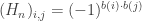
 (H_n)_{i,j} = (-1)^{b(i)\cdot b(j)}, for each i,j such that 0\leq i,j\leq n-1. Inductively, these can be defined by

H_1 = \left( \begin{array}{cc} 1 & 1\\ 1 & -1 \\ \end{array} \right), \ \ \ \ \ \ H_n = \left( \begin{array}{cc} H_{n-1} & H_{n-1}\\ H_{n-1} & -H_{n-1} \\ \end{array} \right), \ \ \ \ \ n>1.
The Walsh-Hadamard transform of f 
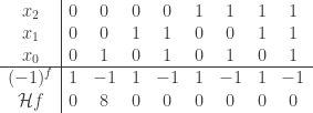
is defined to be the vector in {\mathbb{R}}^{2^n} whose kth component is

({\mathcal{H}} f)(k) = \sum_{i \in \{0,1,\ldots,2^n-1\}}(-1)^{b(i) \cdot b(k) + f(b(i))} = (H_n (-1)^f)_k,

where we define (-1)^f as the column vector where the ith component is

(-1)^f_i = (-1)^{f(b(i))},

for i = 0,\ldots,2^n-1.

Example
A Boolean function of three variables cannot be bent. Let f be defined by:

\begin{array}{c|cccccccc} x_2 & 0 & 0 & 0 & 0 & 1 & 1 & 1 & 1 \\ x_1 & 0 & 0 & 1 & 1 & 0 & 0 & 1 & 1 \\ x_0 & 0 & 1 & 0 & 1 & 0 & 1 & 0 & 1 \\ \hline (-1)^f & 1 & -1 & 1 & -1 & 1 & -1 & 1 & -1 \\ {\mathcal{H}}f & 0 & 8 & 0 & 0 & 0 & 0 & 0 & 0 \\ \end{array}
This is simply the function f(x_0,x_1,x_2)=x_0. It is even because

\Omega_f = \{ (0,0,1), (0,1,1), (1,0,1), (1,1,1) \},\ \mbox{ so } \ \omega = 4.

Here is some Sage code verifying this:

sage: from sage.crypto.boolean_function import *
sage: f = BooleanFunction([0,1,0,1,0,1,0,1])
sage: f.algebraic_normal_form()
x0
sage: f.walsh_hadamard_transform()
(0, -8, 0, 0, 0, 0, 0, 0)

(The Sage method walsh_hadamard_transform is off by a sign from the definition we gave.) We will return to this example later.

Let X=(V,E) be the Cayley graph of f:

V = GF(2)^n,\ \ \ \ E = \{(v,w)\in V\times V\ |\ f(v+w)=1\}.
We shall assume throughout and without further mention that f(0)\not=1, so X has no loops. In this case, X is an \omega-regular graph having r connected components, where

r = |GF(2)^n/{\rm Span}(\Omega_f)|.

For each vertex v\in V, the set of neighbors N(v) of v is given by

N(v)=v+\Omega_f,

where v is regarded as a vector and the addition is induced by the usual vector addition in GF(2)^n. Let A = (A_{ij}) be the 2^n\times 2^n adjacency matrix of X, so

A_{ij} = f(b(i)+b(j)), \ \ \ \ \ 0\leq i,j\leq 2^n-1.

Example:
Returning to the previous example, we construct its Cayley graph.

First, attach afsr.sage from [C] in your Sage session.

     sage: flist = [0,1,0,1,0,1,0,1]
     sage: V = GF(2)ˆ3
     sage: Vlist = V.list()
     sage: f = lambda x: GF(2)(flist[Vlist.index(x)])
     sage: X = boolean_cayley_graph(f, 3)
     sage: X.adjacency_matrix()
     [0 1 0 1 0 1 0 1]
     [1 0 1 0 1 0 1 0]
     [0 1 0 1 0 1 0 1]
     [1 0 1 0 1 0 1 0]
     [0 1 0 1 0 1 0 1]
     [1 0 1 0 1 0 1 0]
     [0 1 0 1 0 1 0 1]
     [1 0 1 0 1 0 1 0]
     sage: X.spectrum()
     [4, 0, 0, 0, 0, 0, 0, -4]
     sage: X.show(layout="circular")

In her thesis, Bernasconi found a relationship between the spectrum of the Cayley graph X,

{\rm Spectrum}(X) = \{\lambda_k\ |\ 0\leq k\leq 2^n-1\},

(the eigenvalues \lambda_k of the adjacency matrix A) to the Walsh-Hadamard transform \mathcal H f = H_n (-1)^f. Note that f and (-1)^f are related by the equation f=\frac 1 2 (e - (-1)^f), where e=(1,1,...,1). She discovered the relationship

\lambda_k = \frac 1 2 (H_n e - \mathcal H f)_k

between the spectrum of the Cayley graph X of a Boolean function and the values of the Walsh-Hadamard transform of the function. Therefore, the spectrum of X, is explicitly computable as an expression in terms of f.

References:

[BC] A. Bernasconi and B. Codenotti, Spectral analysis of Boolean functions as a graph eigenvalue problem, IEEE Trans. Computers 48(1999)345-351.

[CJMP] Charles Celerier, David Joyner, Caroline Melles, David Phillips, On the Hadamard transform of monotone Boolean functions, Tbilisi Mathematical Journal, Volume 5, Issue 2 (2012), 19-35.

[S] P. Stanica, Graph eigenvalues and Walsh spectrum of Boolean functions, Integers 7(2007)\# A32, 12 pages.

Here’s an excellent video of Pante Stanica on interesting applications of Boolean functions to cryptography (30 minutes):

The Vigenère cipher and Sage

The Vigenère cipher is named after Blaise de Vigenère, a sixteenth century diplomat and cryptographer, by a historical accident. Vigene`re actually invented a different and more complicated cipher. The so-called “Vigenère cipher” cipher was actually invented by Giovan Batista Belaso in 1553. In any case, it is this cipher which we shall discuss here first.

This cipher has been re-invented by several authors, such as author and mathematician Charles Lutwidge Dodgson (Lewis Carroll) who claimed his 1868 “The Alphabet Cipher” was unbreakable. Several others claimed the so-called Vigenère cipher was unbreakable (e.g., the Scientific American magazine in 1917). However, Friedrich Kasiski and Charles Babbage broke the cipher in the 1800’s [1]. This cipher was used in the 1700’s, for example, during the American Civil War. The Confederacy used a brass cipher disk to implement the Vigenère cipher (now on display in the NSA Museum in Fort Meade) [1].

The so-called Vigenère cipher is a generalization of the Cesaer shift cipher. Whereas the shift cipher shifts each letter by the same amount (that amount being the key of the shift cipher) the so-called Vigenère cipher shifts a letter by an amount determined by the key, which is a word or phrase known only to the sender and receiver).

For example, if the key was a single letter, such as “C”, then the so-called Vigenère cipher is actually a shift cipher with a shift of 2 (since “C” is the 2-nd letter of the alphabet, if you start counting at 0). If the key was a word with two letters, such as “CA”, then the so-called Vigenère cipher will shift letters in even positions by 2 and letters in odd positions are left alone (or shifted by 0, since “A” is the 0-th letter, if you start counting at 0).

REFERENCES:
[1] Wikipedia article on the Vigenere cipher.

Using Sage, let’s look at a message (a chant at football games between rivals USNA and West Point):

sage: AS = AlphabeticStrings()           
sage: A = AS.alphabet()
sage: VC = VigenereCryptosystem(AS, 1) # sets the key length to be = 1
sage: m = VC.encoding("Beat Army!"); m  # trivial example
BEATARMY

Now, we choose for illustration a simple key of length 1, and encipher this message:

sage: key = AS("D")
sage: c = VC.enciphering(key, m)
sage: c  # a trivial example
EHDWDUPB

You see here that in this case the cipher boils down to the Caesar/shift cipher (shifting by 3).

Deciphering is easy:

sage: VC.deciphering(key, c)
BEATARMY

Next, we choose for illustration a simple key of length 2, and encipher the same message:

sage: VC = VigenereCryptosystem(AS, 2)
sage: key = AS("CA")
sage: m = VC.encoding("Beat Army!"); m
BEATARMY
sage: c = VC.enciphering(key, m); c
DECTCROY

Since one of the key letters is “A” (which shifts by 0), half the plaintext is unchanged in going to the ciphertext.

Here is the algorithmic description of the above (so-called) Vigenère cipher:

    ALGORITHM:
    INPUT: 
      key - a string of upper-case letters (the secret "key")
      m - string of upper-case letters (the "plaintext" message)
    OUTPUT:
      c - string of upper-case letters (the "ciphertext" message)

  Identify the alphabet A, ..., Z with the integers 0, ..., 25. 
    Step 1: Compute from the string key a list L1 of corresponding
            integers. Let n1 = len(L1).
    Step 2: Compute from the string m a list L2 of corresponding
            integers. Let n2 = len(L2).
    Step 3: Break L2 up sequencially into sublists of size n1, and one sublist
            at the end of size <=n1. 
    Step 4: For each of these sublists L of L2, compute a new list C given by 
            C[i] = L[i]+L1[i] (mod 26) to the i-th element in the sublist, 
            for each i.
    Step 5: Assemble these lists C by concatenation into a new list of length n2.
    Step 6: Compute from the new list a string c of corresponding letters.

Once it is known that the key is, say, n characters long, frequency analysis can be applied to every n-th letter of the ciphertext to determine the plaintext. This method is called “Kasiski examination“, or the “Kasiski attack” (although it was first discovered by Charles Babbage).

The cipher Vigenère actually discovered is an “auto-key cipher” described as follows.

ALGORITHM:
    INPUT: 
      key - a string of upper-case letters (the secret "key")
      m - string of upper-case letters (the "plaintext" message)
    OUTPUT:
      c - string of upper-case letters (the "ciphertext" message)

  Identify the alphabet A, ..., Z with the integers 0, ..., 25. 
    Step 1: Compute from the string m a list L2 of corresponding
            integers. Let n2 = len(L2). 
    Step 2: Let n1 be the length of the key. Concatenate the string 
            key with the first n2-n1 characters of the plaintext message.
            Compute from this string of length n2 a list L1 of corresponding
            integers. Note n2 = len(L1).
    Step 3: Compute a new list C given by C[i] = L1[i]+L2[i] (mod 26), for each i.
            Note n2 = len(C).
    Step 5: Compute from the new list a string c of corresponding letters.

Note how the key is mixed with the plaintext to create the enciphering of the plaintext to ciphertext in Steps 2 and 3.

A screencast describing this has been posted to vimeo.