Hans Berliner – a life built around chess

Posted on 2026/02/02 by wdjoyner

Lacking a suitable reference, here is a short bio of this fascinating researcher compiled by claude.

Early Life and Emigration from Germany

Hans Berliner was born in Berlin, Germany in 1929, into a family with a remarkable technological heritage. His great-uncle, Emile Berliner, was the inventor of the gramophone and held the patent on the disc recording format—a technology that would eventually prove superior to Thomas Edison’s cylindrical records and become the ancestor of all subsequent disc-based media formats, including hard drives and modern optical discs. The Berliner family had been involved in telephone technology at the turn of the century, with Emile owning the patent on the carbon receiver for the telephone and establishing a telephone company in Hanover, Germany.

Young Hans entered the German public school system just as Adolf Hitler was rising to power. The first hour of each school day was devoted to “religion” (meaning Christianity) and National Socialism—activities in which Berliner was not permitted to participate. He was also excluded from joining his friends in the Hitler Youth. “I was told that I was Jewish, and they didn’t want me,” Berliner later recalled. “That was quite a shock, and I guess that’s one of those things that sort of grows you up a little bit.”

Despite the oppressive political atmosphere, Germany in the 1930s remained a stimulating environment for a child interested in science. Berliner remembered it as “probably the best place in the world” for such interests. “The Germans were full of inventiveness and managed to produce things that were very, very good,” he recalled. He particularly remembered a metal wind-up toy car equipped with a working servomechanism that could sense when it was about to run off a ledge and automatically steer away—a sophisticated device for a child’s toy in 1935. German kindergarteners were reportedly “three years ahead” of their American counterparts in mathematics, and these formative years had a lasting positive effect on Berliner’s intellectual development.

The family’s fortunes changed dramatically in 1936 when two visitors from the United States came to stay with the Berliners. Seven-year-old Hans soon learned that the family would be leaving Germany. A nephew of Uncle Emile, Joseph Sanders, had arranged for approximately ten members of the extended family to emigrate to America. In 1937, the Berliner family arrived in the Washington, D.C. area, speaking very little English and with thick German accents.

Berliner’s father held a master’s degree in electrical engineering, while his mother had essentially no education beyond high school. Berliner would later describe his home environment as not particularly intellectual, with his parents “more just interested in surviving.” However, one of the most formative experiences of his life occurred before he was three years old, when his grandmother gave him a chalkboard with letters and numbers around the edges. He began making words and doing sums, and from that point on, learning came naturally. “I just wanted to know everything about everything,” he recalled.

Education and the Discovery of Chess

Berliner doggedly pursued his studies at Henry D. Cooke Elementary School in Washington, eventually graduating with the top grammar marks in his class. One of his fellow students was Carlos Fuentes, who would become a famous Mexican novelist and essayist. Fuentes vividly remembered Berliner as the “extremely brilliant boy” with “deep-set, bright eyes—a brilliant mathematical mind—and an air of displaced courtesy that infuriated the popular, regular, feisty, knickered, provincial, Depression-era sons-of-bitches.”

At age 11 and 12, Berliner read every book in the adult section of the library about astronomy, developing what he felt was phenomenal knowledge of the subject. He even reached the point where he recognized that certain theories about the formation of the solar system were patently wrong because they violated physical principles he understood. However, there was no outlet for such precocious knowledge—no school could handle a 12-year-old with advanced expertise, and no special programs existed for gifted children at that time.

Into this intellectual vacuum came chess. At age 13, Berliner was at a summer camp when rain forced everyone indoors. He noticed other children playing a game on a board that wasn’t checkers. He asked about the rules, learned them, and by the end of the day was already beating one of the other players. “Chess seemed a natural,” he recalled. “In a way, I sometimes thought maybe that was not the best path to go, but that was the one that presented itself.” Chess offered something that astronomy could not: a domain where a young person could immediately compete in the adult world.

Berliner progressed rapidly in chess, becoming a master by 1949 or 1950. He would later represent the United States at the 10th Chess Olympiad in Helsinki, Finland in 1952, where he met his future wife, a Finnish woman whom he married in 1954.

Academic and Professional Struggles

After high school, Berliner entered George Washington University to pursue a degree in physics with ambitions of becoming a top-notch physicist. However, he had no understanding of the academic path required—the need for a Ph.D. and years of study. He was one of the top physics students, but he grew bored with the program and began “majoring in bridge” rather than attending classes. Before long, his grades had plummeted, and the draft beckoned. He entered the U.S. Army in early 1951 and served with the German occupation forces. Throughout his tour of duty, Berliner continued to play chess, including one exhibition where he simultaneously played eight games against one of the top German teams—and won them all.

Upon his return to civilian life, Berliner was reluctant to return to college. It was Isador Turover, a fellow European immigrant and former top U.S. chess player who had become a successful lumber magnate in Washington, who set Berliner straight. Turover, whom Berliner had met through chess circles, told the younger man in no uncertain terms, “You will finish your degree.” He hired Berliner into his lumber company so he could earn money to pay his way through college, since there was no family money for education and Berliner had never secured a scholarship.

Unable to return to physics due to his low grade point average, Berliner switched to psychology, naively believing that with a psychology degree he could “hang out a shingle as a psychologist and start counseling people.” Again fate intervened. A classmate who worked at the Naval Research Laboratory told Berliner, “We need people like you where I work.” This led to a position in what was then called “human engineering” or “engineering psychology”—a predecessor to modern interface design and human factors research.

Early Career and First Encounters with Computers

Starting at the Naval Research Laboratory in 1954, Berliner worked on human engineering problems, such as ensuring that Navy pilots didn’t pull the wrong lever and eject themselves when trying to lower the landing gear. During this period, he had his first brush with computers. A colleague at the lab was helping to build NRL’s own computer—one of very few computers in existence at that time—and suggested they might write a chess program together. They talked about it and even did a few preliminary things, but the project never got off the ground. Berliner had read the foundational articles by Claude Shannon and by Newell and Simon about computer chess in Scientific American, but he “didn’t have the foggiest notion how to implement it.”

From the Naval Research Lab, Berliner moved to Martin Company in Denver, then to General Electric’s Missile and Space Vehicle Division in Valley Forge, Pennsylvania—which he described as “one of the finest places I’ve ever operated,” with more talented people than perhaps even Carnegie Mellon—and finally to IBM in Bethesda, Maryland. Throughout these moves, his specialty remained human factors work, which he did not consider particularly fulfilling. “My pay was skyrocketing, but I had an awful lot of spare time,” he later recalled.

Rise to Chess Prominence

hroughout the 1950s, Berliner’s chess ranking continued to climb. He became a Senior Master with a rating in the 2420-2440 range, placing him among the top ten players in the United States. He played regularly in the U.S. Invitational Championship, and in the year Bobby Fischer won the title for the first time, Berliner finished fifth and drew with Fischer.

His reputation became especially strong in correspondence chess—games played through the mail—where his systematic approach and analytical mind could shine without the time pressure of tournament play. From 1965 to 1968, Berliner served as World Correspondence Chess Champion, winning his first championship with a remarkable record of 12 wins and 4 draws in 16 games, a margin of victory three times better than any previous champion. He remained the top-ranked U.S. correspondence chess player until 2005, long after he stopped competing.

Murray Campbell, who would later work on IBM’s Deep Blue, observed that Berliner wasn’t a “star” player in the mold of Bobby Fischer or Garry Kasparov, but achieved chess greatness “using a very systematic approach and a lot of hard work.” Berliner “had competitive fire” and an analytical mind that enabled him to beat players “who might very well have been more talented than him.”

Carnegie Mellon and Computer Chess Research

While at IBM in the late 1960s, Berliner began thinking seriously about computer chess. He had never written a program in his life, so he had to learn programming while developing his first chess program. Called “J. Biit” (an acronym for “Just Because It Is There”), it was written in PL/1 and played in the first U.S. Computer Chess Championship in 1970, finishing around the middle of the field.

In 1967, Berliner met future Nobel laureate Herbert Simon at a technical meeting. Simon, who in 1956 had famously predicted that within ten years a computer would become world chess champion, was still interested in chess-playing computers. He offered Berliner a job at Carnegie Mellon University, but Berliner turned down the position of researcher. “If I’m going to come there, you’ve got to put me on the student track,” he insisted. At nearly 40 years old, feeling that he wanted to do “something worthwhile” with his life, Berliner was accepted into CMU’s Computer Science Department as a doctoral student in 1969.

Berliner found CMU to be a “good” but “chaotic” environment, with the department “up on wobbly feet.” The founding department head, Alan Perlis, was “an amazing, wonderful person” with “a desire for progress and truth that was very, very commendable.” Newell allowed Berliner to begin his thesis work on computer chess even before completing the rigorous qualifying examinations.

For his doctoral dissertation, titled “Chess as Problem Solving,” Berliner developed a chess program called CAPS that incorporated what he called the “causality facility.” This mechanism dragged back descriptions of tactical events through the search tree, allowing the program to reason about why certain moves failed and what characteristics a move would need to prevent similar failures. The program could figure out how to block threats without trying every possibility, simply by reasoning about what was required.

However, even as Berliner refined CAPS, he became convinced that rule-based approaches had fundamental limitations. “I had a set of rules that were limited,” he explained. “They were the most important things—maybe 80 percent—but that’s nothing. The other 20 percent includes the things the top players know how to do. That’s why they’re the top players.” Newell and Simon kept encouraging him to create more rules, but Berliner recognized that something crucial was missing: the intuitive understanding that allowed grandmasters to evaluate positions at a glance.

The B* Algorithm and Backgammon

While searching for new research directions, Berliner learned backgammon from his father-in-law and decided to write a program for this simpler game. His initial attempts encountered a familiar problem: the program would reach a certain point and then bog down, “trying to optimize things that it should have forgotten about.” At some point, when a player was clearly winning, the strategy should change—the program needed to recognize when transitions were coming.

Berliner hit upon the idea of using fuzzy logic—still a novel concept in the 1970s—to assign different rules “weights” or “application factors” based on their relative importance at each stage of the game. The resulting program, called BKG, began winning games it would have previously lost. In July 1979, BKG became the first computer program to defeat a reigning world champion in any board game when it beat backgammon champion Luigi Villa.

One of the highlights of Berliner’s research was the B* (“B-star”) algorithm, designed to emulate what he called the “jumping around” process in human thought. Rather than using traditional best-first or depth-first searches with arbitrary termination criteria, B* assigned an “optimistic” and a “pessimistic” score to each node. The algorithm continued searching a branch as long as the pessimistic value of the best node was no worse than the optimistic value of its sibling nodes. B* found paths that were sufficient for a task rather than theoretically “perfect” ones—emulating how a human chess master stops searching when finding a move that seems clearly best.

As Andy Palay, one of Berliner’s students, observed, B* represented “a much more directed search toward what appear to be the most promising paths” compared to simple best-first searches.

HiTech: A Chess-Playing Machine

In 1983, Berliner embarked on what he would later describe as one of the best periods of his professional life. His student Carl Ebeling proposed building a chess-playing machine using the then-novel technology of very-large-scale integrated (VLSI) circuits. Ebeling custom-designed a processor to generate chess moves, and the resulting machine, named HiTech, used 64 of these processors—one for each square of the chessboard—operating in parallel.

The enthusiasm for HiTech was extraordinary. “Everyone wanted to know what the latest developments were, and if they could help,” Berliner recalled. Volunteers from inside and outside CMU’s Computer Science Department took turns wire-wrapping connections in a third-floor lab in Wean Hall. With a hardware budget of only about five thousand dollars, the team scavenged parts and bought 32K memory chips at twenty or thirty dollars each.

A working prototype was completed in 1984. HiTech could consider 175,000 positions per second—compared to the one or two moves per second a top human player might examine. The machine also incorporated pattern recognizers that Ebeling designed to identify specific positional features, such as trapped bishops, pawn structures, and king safety issues. These pattern recognizers “sat like gargoyles on the edge of the thing watching the positions go by,” detecting problems and opportunities that pure calculation might miss.

“From the very beginning, I could see that it had the potential—maybe not every single time—it had the potential to play better than any device that existed,” Berliner recalled. The team worked hundred-hour weeks, with Monday morning meetings to discuss progress and problems. “Every week it got better. Every week the machine played better than it did the week before; now that’s incredible, that’s truly amazing.”

In October 1985, HiTech won Pittsburgh’s Gateway Open chess competition, earning the rank of “master.” That same year it won the ACM tournament for chess programs. The machine went on to win the Pennsylvania State Championship three consecutive years—something Berliner himself had never achieved as a human player. By 1987, HiTech was ranked 190th in the United States and was the only computer among the top 1,000 players, with a rating around 2440—Senior Master level.

One particularly memorable achievement was a four-game match against grandmaster Arnold Denker, which HiTech won 3.5 to 0.5. “It outplayed him in every game, in every single game. It completely beat him,” Berliner recalled.

Rivalry and the Road to Deep Blue

While Berliner’s team was developing HiTech, fellow CMU graduate students Feng-hsiung Hsu and Thomas Anantharaman began work on another chess-playing computer called ChipTest. Like HiTech, it relied on VLSI technology, but it was significantly faster—by 1987, ChipTest was searching 500,000 moves per second.

Daniel Sleator, a CMU professor who had founded the Internet Chess Club, noted that having two competing chess systems developed simultaneously at CMU “reflects a number of important things about the culture in the Computer Science Department. For one thing, there is a tremendous amount of respect for the work of graduate students. The faculty gives them the benefit of the doubt, and in many cases, including this one, it pays off.”

However, the relationship between the teams deteriorated over time. “There was some tension that never got resolved, and there were some hard feelings in terms of the competition between the two groups,” Campbell acknowledged. ChipTest evolved into Deep Thought, which won the World Computer Chess Championship in 1989. IBM subsequently hired Hsu, Campbell, and Anantharaman, and the machine that became Deep Blue eventually defeated world champion Garry Kasparov in 1997.

Legacy and Perspective

In retrospect, Berliner was characteristically blunt about the field he helped pioneer. Computer chess was “a research dead-end” as far as artificial intelligence was concerned, he concluded. “The whole AI thesis was wrong. AI researchers thought more knowledge would do everything.” Instead, more powerful processors and machine-learning techniques powered by statistical analysis, rather than human-devised rules, proved capable of cracking data-intensive problems in speech, image analysis, and data retrieval.

However, those who studied Berliner’s work disagreed with his self-assessment. “He covered a lot of ground, and he achieved excellence in all of those areas,” said Campbell. Jonathan Schaeffer, a professor at the University of Alberta who led the team that created the unbeatable Chinook checkers program, noted that Berliner “has a legacy of excellent papers that contain insights, algorithms and new ideas that aren’t as common today as they should be. People continue to reference his work when they realize there are other ways to do things, and then they point at Hans.”

Schaeffer observed that “most scientists aren’t willing to take the kinds of risks that Hans would take. But that’s why his papers are still around, while the papers of his contemporaries are long gone and forgotten.”

Berliner’s willingness to question conventional wisdom led to controversy, including his accusation that Russian computer scientist and chess grandmaster Mikhail Botvinnik had committed fraud by manipulating published results. Schaeffer and others reviewed Berliner’s evidence and concluded that Botvinnik had indeed massaged his results. Similarly, Berliner’s 1999 book The System: A World Champion’s Approach to Chess attracted sharp criticism from some reviewers, but the attacks left him unbowed.

His former students remembered not just his demanding standards but his generosity. “Working with Hans was a lot of fun,” recalled Palay. “There was a great deal of graciousness, both on a personal level and a professional level. He was very much concerned with making sure that he was treating me well, not just as his student, but as a person.” Ebeling noted that Berliner “led by example more than anything else. There was a constant attention to detail, and he was always thinking, looking out for the next idea that might work.”

Berliner retired from Carnegie Mellon in 1998. His advice to students: “Learn all the substantive knowledge that you can. In the final analysis, all knowledge hangs together, and the more you know, the easier it will be to make good decisions in the future. Learn something that has value—something quantitative, hopefully. Have something you can do that someone else will want to pay you for—a product. If you don’t have that, it’s going to be tough for you.”

Hans Berliner passed away on January 13, 2017, at the age of 87, leaving behind a remarkable legacy as a world chess champion, a pioneer in computer game-playing, and a scientist who was never afraid to challenge conventional wisdom in pursuit of truth.

Main References

Interview with Gardner Hendrie on 2005-03-07, Oral history of Hans Berliner, CHM Reference number X3131.2005, Computer History Museum, 2005.

J. Togyer, The Iconoclast, in The Link: The Magazine of the Carnegie Mellon University School of Computer Science, May 7, 2012.

The shell algorithm and a new book

Posted on 2026/01/06 by wdjoyner

A Peek Behind the Curtain

One feature of my forthcoming book with Caroline Melles, Exploring Graphs via Harmonic Morphisms, is its computational emphasis. Many of the examples and insights emerged not from pure contemplation, but from extensive experimentation using SageMath. This post gives a glimpse into the algorithmic machinery that made this exploration possible.

The fundamental problem I faced in generating examples was this: given two graphs Γ₁ and Γ₂, find all harmonic morphisms φ: Γ₂ → Γ₁. This approach is direct—a brute force algorithm that constructs all possible “color lists” (vertex labelings that encode potential morphisms) and tests each one for the harmonic property. Straightforward? Yes. Fast? Definitely not.

However, when the target graph Γ₁ is a path graph, one can do better. The “shell algorithm” exploits the geometry of distance in the source graph. Starting from a chosen vertex v₀, one builds outward through successive neighborhoods—vertices at distance 1, then 2, and so on—assigning colors constrained by distance from the starting point. At each stage, one checks necessary conditions before proceeding, pruning impossible branches early. The automorphism groups of both graphs then generate equivalent colorings, and after removing duplicates, one has a complete enumeration of the harmonic morphisms.

That’s what was done for various choices of small graphs, printing computational data to a file whose name used notation or terminology for the graphs $\Gamma_1$ and $\Gamma_2$ . Months of computer searches resulted in a number of conjectures that were used to shape the material in the book.

Shanks’ SQUFOF according to McMath

Posted on 2021/07/30 by wdjoyner

In 2003, a math major named Steven McMath approached Fred Crabbe and I about directing his Trident thesis. (A Trident is like an honors thesis, but the student gets essentially the whole year to focus on writing the project.) After he graduated, I put a lot of his work online at the USNA website. Of course, I’ve retired since then and the materials were removed. This blog post is simply to try to repost a lot of the materials which arose as part of his thesis (which are, as official works of the US government, all in the public domain; of course, Dan Shanks notes are copyright of his estate and are posted for scholarly use only).

McMath planned to study Dan Shanks‘ SQUFOF method, which he felt could be exploited more than had been so far up to that time (in 2004). This idea had a little bit of a personal connection for me. Dan Shanks was at the University of Maryland during the time (1981-1983) I was a grad student there. While he and I didn’t talk as much as I wish we had, I remember him as friendly guy, looking a lot like the picture below, with his door always open, happy to discuss mathematics.

One of the first things McMath did was to type up the handwritten notes we got (I think) from Hugh Williams and Duncan Buell. A quote from a letter from Buell:

“Dan probably invented SQUFOF in 1975. He had just bought an HP 67 calculator, and the algorithm he invented had the advantages of being very simple to program, so it would fit on the calculator, very powerful as an algorithm when measured against the size of the program, and it factors double precision numbers using single precision arithmetic.“

Here are some papers on this topic (with thanks to Michael Hortmann for the references to Gower’s papers):

David Joyner, Notes on indefinite integral binary quadratic forms with SageMath, preprint 2004. pdf

F. Crabbe, D. Joyner, S. McMath, Continued fractions and Parallel SQUFOF, 2004. arxiv

D. Shanks, Analysis and Improvement of the Continued Fraction Method of Factorization, handwritten notes 1975, typed into latex by McMath 2004. pdf.

D. Shanks, An Attempt to Factor N = 1002742628021, handwritten notes 1975, typed into latex by McMath 2004. pdf.

D. Shanks, SQUFOF notes, handwritten notes 1975, typed into latex by McMath 2004. pdf.

S. McMath, Daniel Shanks’ Square Forms Factorization, 2004 preprint. pdf1, pdf2.

S. McMath, Parallel Integer Factorization Using Quadratic Forms, Trident project, 2004. pdf.

Since that time, many excellent treatments of SQUFOF have been presented. For example, see

J. Gower, S. Wagstaff, Square Form Factorization, Math Comp, 2008. pdf.

J. Gower, Square Form Factorization, PhD Thesis, December 2004. pdf.

How do I construct … in GAP?

Posted on 2017/08/09 by wdjoyner

This page is devoted to answering some basic questions along the line “How do I construct … in GAP?” You may view the html source code for the GAP commands without the output or GAP prompt.

Please send suggestions, additions, corrections to David Joyner.

This page itself is under construction…

Questions

How do I construct a … group? permutation dihedral cyclic conjugacy classes of a finitely presented	How do I … a polynomial? factor find roots of evaluate Groebner basis of ideal of
Brauer characters	How do I find the … of a group representation? character table
How do I compute an mod m, where A is …? an integer a square matrix a polynomial	Given a group G, how do I compute … ? all normal subgroups of G all abelian subgroups of G a homomorphism from G to another group H the semi-direct product of G with another group H all groups of order 12 written as semi-direct products the cohomology of G with coefficients in A

Answers

- permutation:
  To construct a permutation group, write down generators in disjoint cycle notation, put them in a list (i.e., surround them by square brackets), and the permutation group G generated by the cycles (1,2)(3,4) and (1,2,3):

gap> G:=Group((1,2)(3,4),(1,2,3));

Group([ (1,2)(3,4), (1,2,3) ])

This is of course a subgroup of the symmetric group S₄ on 4 letters. Indeed, this G is in fact the alternating group on four letters, A₄.

By virtue of the fact that the permutations generating G employ integers less than or equal to 4, this group G is a subgroup of the symmetric group S₄ on 4 letters. Some permutation groups have special constructions:

gap> S4:=SymmetricGroup(4);
Sym( [ 1 .. 4 ] )
gap> A4:=AlternatingGroup(4);
Alt( [ 1 .. 4 ] )
gap> IsSubgroup(S4,G);
true
gap> IsSubgroup(A4,G);
true
gap> S3:=SymmetricGroup(3);
Sym( [ 1 .. 3 ] )
gap> IsSubgroup(S3,G);
false

- dihedral
  To construct a dihedral group, use the special “DihedralGroup” command:

gap> G:=DihedralGroup(6);
gap> Size(G);
6
gap> f:=GeneratorsOfGroup( G );
[ f1, f2 ]
gap> f[1]^2; f[2]^3;
identity of ...
identity of ...
gap> f[1]^2= f[2]^3;
true

cyclic group
To construct a cyclic group, you may construct integers mod n:

gap> R:=ZmodnZ( 12);
(Integers mod 12)
gap> a:=Random(R);
ZmodnZObj( 11, 12 )
gap> 4*a;
ZmodnZObj( 8, 12 )
gap> b:=Random(R);
ZmodnZObj( 9, 12 )
gap> a+b;
ZmodnZObj( 8, 12 )

or use the special “CyclicGroup” command

gap> G:=CyclicGroup(12);
pc group of size 12 with 3 generators
gap> a:=Random(G);
f3^2
gap> f:=GeneratorsOfGroup( G );
[ f1, f2, f3 ]
gap> f[1]^4;
f3
gap> f[1]^12;
identity of ...

conjugacy:
The conjugacy classes of a group G are computed using the “ConjugacyClasses” command. This is a list of classes {x^-1*g*x | x in G}.

gap> G:=SL(2,7);
SL(2,7)
gap> CG:=ConjugacyClasses(G);
[ [ [ Z(7)^0, 0*Z(7) ], [ 0*Z(7), Z(7)^0 ] ]^G,
  [ [ 0*Z(7), Z(7)^3 ], [ Z(7)^0, Z(7)^5 ] ]^G,
  [ [ 0*Z(7), Z(7)^4 ], [ Z(7)^5, Z(7)^5 ] ]^G,
  [ [ Z(7)^3, 0*Z(7) ], [ 0*Z(7), Z(7)^3 ] ]^G,
  [ [ 0*Z(7), Z(7)^3 ], [ Z(7)^0, Z(7)^2 ] ]^G,
  [ [ 0*Z(7), Z(7)^4 ], [ Z(7)^5, Z(7)^2 ] ]^G,
  [ [ 0*Z(7), Z(7)^3 ], [ Z(7)^0, 0*Z(7) ] ]^G,
  [ [ 0*Z(7), Z(7)^3 ], [ Z(7)^0, Z(7)^4 ] ]^G,
  [ [ 0*Z(7), Z(7)^3 ], [ Z(7)^0, Z(7) ] ]^G,
  [ [ Z(7)^4, 0*Z(7) ], [ 0*Z(7), Z(7)^2 ] ]^G,
  [ [ Z(7)^5, 0*Z(7) ], [ 0*Z(7), Z(7) ] ]^G ]
gap> g:=Representative(CG[3]); Order(g);
[ [ 0*Z(7), Z(7)^4 ], [ Z(7)^5, Z(7)^5 ] ]
14
gap> g:=Representative(CG[4]); Order(g);
[ [ Z(7)^3, 0*Z(7) ], [ 0*Z(7), Z(7)^3 ] ]
2
gap> g:=Representative(CG[5]); Order(g);
[ [ 0*Z(7), Z(7)^3 ], [ Z(7)^0, Z(7)^2 ] ]
7
gap> g:=Representative(CG[6]); Order(g);
[ [ 0*Z(7), Z(7)^4 ], [ Z(7)^5, Z(7)^2 ] ]
7
gap>

presented
To construct a finitely presented group in GAP, use the “FreeGroup” and “FpGroupPresentation” commands. Here is one example.

gap> M12 := MathieuGroup( 12 );
Group([ (1,2,3,4,5,6,7,8,9,10,11), (3,7,11,8)(4,10,5,6), (1,12)(2,11)(3,6)(4,8)(5,9)(7,10) ])
gap> F := FreeGroup( "a", "b", "c" );
free group on the generators [ a, b, c ]
gap> words := [ F.1, F.2 ];
[ a, b ]
gap> P := PresentationViaCosetTable( M12, F, words );
presentation with 3 gens and 10 rels of total length 97
gap> TzPrintRelators( P );
#I  1. c^2
#I  2. b^4
#I  3. a*c*a*c*a*c
#I  4. a*b^2*a*b^-2*a*b^-2
#I  5. a^11
#I  6. a^2*b*a^-2*b^2*a*b^-1*a^2*b^-1
#I  7. a*b*a^-1*b*a^-1*b^-1*a*b*a^-1*b*a^-1*b^-1
#I  8. a^2*b*a^2*b^2*a^-1*b*a^-1*b^-1*a^-1*b^-1
#I  9. a*b*a*b*a^2*b^-1*a^-1*b^-1*a*c*b*c
#I  10. a^4*b*a^2*b*a^-2*c*a*b*a^-1*c
gap> G := FpGroupPresentation( P );
fp group on the generators [ a, b, c ]
gap> RelatorsOfFpGroup( G );  
[ c^2, b^4, a*c*a*c*a*c, a*b^-2*a*b^-2*a*b^-2, a^11, a^2*b*a^-2*b^-2*a*b^-1*a^2*b^-1, a*b*a^-1*b*a^-1*b^-1*a*b*a^-1*b*a^-1*b^-1,
  a^2*b*a^2*b^-2*a^-1*b*a^-1*b^-1*a^-1*b^-1, a*b*a*b*a^2*b^-1*a^-1*b^-1*a*c*b*c, a^4*b*a^2*b*a^-2*c*a*b*a^-1*c ]
gap> Size(M12);
95040
gap> Size(G);
95040
gap> IsomorphismGroups(G,M12); 
????????

The last command is computationally intensive and requires more than the default memory allocation of 256M of RAM.

Here is another example.

gap> F := FreeGroup( "a", "b");
free group on the generators [ a, b ]
gap> G:=F/[F.1^2,F.2^3,F.1*F.2*F.1^(-1)*F.2^(-1)];
fp group on the generators [ a, b ]
gap> Size(G);
6

rref
The key command for row reduction is “TriangulizeMat”. The following example illustrates the syntax.

gap> M:=[[1,2,3,4,5],[1,2,1,2,1],[1,1,0,0,0]];
[ [ 1, 2, 3, 4, 5 ], [ 1, 2, 1, 2, 1 ], [ 1, 1, 0, 0, 0 ] ]
gap> TriangulizeMat(M);
gap> M;
[ [ 1, 0, 0, -1, 1 ], [ 0, 1, 0, 1, -1 ], [ 0, 0, 1, 1, 2 ] ]
gap> Display(M);
[ [   1,   0,   0,  -1,   1 ],
  [   0,   1,   0,   1,  -1 ],
  [   0,   0,   1,   1,   2 ] ]
gap> M:=Z(3)^0*[[1,2,3,4,5],[1,2,1,2,1],[1,1,0,0,0]];
[ [ Z(3)^0, Z(3), 0*Z(3), Z(3)^0, Z(3) ],
  [ Z(3)^0, Z(3), Z(3)^0, Z(3), Z(3)^0 ],
  [ Z(3)^0, Z(3)^0, 0*Z(3), 0*Z(3), 0*Z(3) ] ]
gap> TriangulizeMat(M);
gap> Display(M);
 1 . . 2 1
 . 1 . 1 2
 . . 1 1 2
gap>

kernel:
There are different methods for matrices over the integers and matrices over a field. For integer entries, related commands include “NullspaceIntMat” and “SolutionNullspaceIntMat” in section 25.1 “Linear equations over the integers and Integral Matrices” of the reference manual.

gap> M:=[[1,2,3],[4,5,6],[7,8,9]];
[ [ 1, 2, 3 ], [ 4, 5, 6 ], [ 7, 8, 9 ] ]
gap> NullspaceIntMat(M);
[ [ 1, -2, 1 ] ]
gap> SolutionNullspaceIntMat(M,[0,0,1]);
[ fail, [ [ 1, -2, 1 ] ] ]
gap> SolutionNullspaceIntMat(M,[0,0,0]);
[ [ 0, 0, 0 ], [ [ 1, -2, 1 ] ] ]
gap> SolutionNullspaceIntMat(M,[1,2,3]);
[ [ 1, 0, 0 ], [ [ 1, -2, 1 ] ] ]

Here (0,0,1) is not in the image of M
(under v-> v*M) but (0,0,0) and (1,2,3) are.

For field entries, related commands include “NullspaceMat” and “TriangulizedNullspaceMat” in section 24.6 “Matrices Representing Linear Equations and the Gaussian Algorithm”
of the reference manual.

gap> M:=[[1,2,3],[4,5,6],[7,8,9]];
[ [ 1, 2, 3 ], [ 4, 5, 6 ], [ 7, 8, 9 ] ]
gap> NullspaceMat(M);
[ [ 1, -2, 1 ] ]
gap> TriangulizedNullspaceMat(M);
[ [ 1, -2, 1 ] ]
gap> M:=[[1,2,3,1,1],[4,5,6,1,1],[7,8,9,1,1],[1,2,3,1,1]];
[ [ 1, 2, 3, 1, 1 ], [ 4, 5, 6, 1, 1 ], [ 7, 8, 9, 1, 1 ], 
  [ 1, 2, 3, 1, 1 ] ]
gap> NullspaceMat(M);
[ [ 1, -2, 1, 0 ], [ -1, 0, 0, 1 ] ]
gap> TriangulizedNullspaceMat(M);
[ [ 1, 0, 0, -1 ], [ 0, 1, -1/2, -1/2 ] ]

characteristic polynomial:
Please see section 24.12.1 of the GAP reference manual for examples of characteristic polynomial of a square matrix (“CharacteristicPolynomial”) and section 56.3 for examples of the “characteristic polynomial” (called a “TracePolynomial”) of an element of a field extension.

character:
GAP contains very extensive character theoretic functions and data libraries (including an interface the character table in the Atlas). Here is just one simple example.

gap> G:=Group((1,2)(3,4),(1,2,3));
Group([ (1,2)(3,4), (1,2,3) ])
gap> T:=CharacterTable(G);
CharacterTable( Alt( [ 1 .. 4 ] ) )
gap> Display(T);
CT1

     2  2  2  .  .
     3  1  .  1  1

       1a 2a 3a 3b
    2P 1a 1a 3b 3a
    3P 1a 2a 1a 1a

X.1     1  1  1  1
X.2     1  1  A /A
X.3     1  1 /A  A
X.4     3 -1  .  .

A = E(3)^2
  = (-1-ER(-3))/2 = -1-b3
gap> irr:=Irr(G);
[ Character( CharacterTable( Alt( [ 1 .. 4 ] ) ), [ 1, 1, 1, 1 ] ),
  Character( CharacterTable( Alt( [ 1 .. 4 ] ) ), [ 1, 1, E(3)^2, E(3) ] ),
  Character( CharacterTable( Alt( [ 1 .. 4 ] ) ), [ 1, 1, E(3), E(3)^2 ] ),
  Character( CharacterTable( Alt( [ 1 .. 4 ] ) ), [ 3, -1, 0, 0 ] ) ]
gap> Display(irr);
[ [       1,       1,       1,       1 ],
  [       1,       1,  E(3)^2,    E(3) ],
  [       1,       1,    E(3),  E(3)^2 ],
  [       3,      -1,       0,       0 ] ]
gap> chi:=irr[2]; gamma:=CG[3]; g:=Representative(gamma); g^chi;
Character( CharacterTable( Alt( [ 1 .. 4 ] ) ), [ 1, 1, E(3)^2, E(3) ] )
(1,2,3)^G
(1,2,3)
E(3)^2

For further details and examples, see chapters 69– 72 of the GAP reference manual.

brauer:
Just a simple example of what GAP can do here. To construct a Brauer character table:

gap> G:=Group((1,2)(3,4),(1,2,3));
Group([ (1,2)(3,4), (1,2,3) ])
gap> irr:=IrreducibleRepresentations(G,GF(7));
[ [ (1,2)(3,4), (1,2,3) ] -> [ [ [ Z(7)^0 ] ], [ [ Z(7)^0 ] ] ],
  
[ (1,2)(3,4), (1,2,3) ] -> [ [ [ Z(7)^0 ] ], [ [ Z(7)^4 ] ] ],
  
[ (1,2)(3,4), (1,2,3) ] -> [ [ [ Z(7)^0 ] ], [ [ Z(7)^2 ] ] ],
  
[ (1,2)(3,4), (1,2,3) ] -> [
      
[ [ 0*Z(7), Z(7)^3, Z(7)^0 ], [ 0*Z(7), Z(7)^3, 0*Z(7) ], 
[ Z(7)^0, Z(7)^3, 0*Z(7) ] ],
      [ [ 0*Z(7), Z(7)^0, 0*Z(7) ], 
[ 0*Z(7), 0*Z(7), Z(7)^0 ], [ Z(7)^0, 0*Z(7), 0*Z(7) ] ]
     
] ]
gap> brvals := List(irr,chi-> List(ConjugacyClasses(G),c->
BrauerCharacterValue(Image(chi, Representative(c)))));
[ [ 1, 1, 1, 1 ], [ 1, 1, E(3)^2, E(3) ], [ 1, 1, E(3), E(3)^2 ], 
[ 3, -1, 0, 0 ] ]
gap> Display(brvals);
[ [       1,       1,       1,       1 ],
  
[       1,       1,  E(3)^2,    E(3) ],
  
[       1,       1,    E(3),  E(3)^2 ],
  
[       3,      -1,       0,       0 ] ]
gap>

List(ConjugacyClasses(G),c->BrauerCharacterValue(Image(chi, Representative(c)))));
#Display(brvals);
T:=CharacterTable(G);
Display(T);
–>

polynomial
There are various ways to construct a polynomial in GAP.

gap> Pts:=Z(7)^0*[1,2,3];
[ Z(7)^0, Z(7)^2, Z(7) ]
gap> Vals:=Z(7)^0*[1,2,6];
[ Z(7)^0, Z(7)^2, Z(7)^3 ]
gap> g:=InterpolatedPolynomial(GF(7),Pts,Vals);
Z(7)^5*x_1^2+Z(7)

Or:

gap> p:=3;; F:=GF(p);;
gap> R:=PolynomialRing(F,["x1","x2"]);
PolynomialRing(..., [ x1, x2 ])
gap> vars:=IndeterminatesOfPolynomialRing(R);;
gap> x1:=vars[1]; x2:=vars[2];
x1
x2
gap> p:=x1^5-x2^5;
x1^5-x2^5
gap> DivisorsMultivariatePolynomial(p,R);
[ x1^4+x1^3*x2+x1^2*x2^2+x1*x2^3+x2^4, x1-x2 ]

Or:

gap> x:=X(Rationals);
x_1
gap> f:=x+x^2+1;
x_1^2+x_1+1
gap> Value(f,[x],[1]);
3

factor
To factor a polynomial in GAP, there is one command for univariate polynomials (“Factors”) and another command for multivariate polynomials (“DivisorsMultivariatePolynomial”). For a factoring a univariate polynomial, GAP provides only methods over finite fields and over subfields of cyclotomic fields. Please see the examples given in section 64.10 “Polynomial Factorization” for more details. For multivariate polynomials, a very slow algorithm has been implemented in GAP and an interface to a very fast algorithm in Singular has been implemented for those who have both Singular and the GAP Singular package installed. The former of these was illustrated above in “polynomial” above. (Again, the ground field must be a finite field or a subfields of cyclotomic fields.) For the latter, please see the example in the (GAP-)Singular manual FactorsUsingSingularNC.
roots
There are some situations where GAP can find the roots of a polynomial but GAP does not do this generally. (The roots must generate either a finite field or a subfield of a cyclotomic field.) However, there is a package called RadiRoot which must be installed which does help to do this for polynomials with rational coefficients (radiroot itself requires other packages to be installed; please see the webpage for more details). The “Factors” command actually has an option which allows you to increase the groundfield so that a factorization actually returns the roots. Please see the examples given in section 64.10 “Polynomial Factorization” for more details. Here is a second approach.
```
gap> p:=3; n:=4; F:=GF(p^n); c:=Random(F); r:=2;
3
4
GF(3^4)
Z(3^4)^79
2
gap>  x:=X(F,1); f:=x^r-c*x+c-1;
x_1
x_1^2+Z(3^4)^39*x_1+Z(3^4)^36
gap>  F_f:=FieldExtension( F, f );
AsField( GF(3^4), GF(3^8) )
gap>  alpha:=RootOfDefiningPolynomial(F_f);
Z(3^4)^36
gap> Value(f,[x],[alpha]);
0*Z(3)
```
Here is a third. First, enter the following program
```
RootOfPolynomial:=function(f,R)
 local F0,Ff,a;
 F0:=CoefficientsRing(R);
 Ff:=FieldExtension(F0,f);
 a:=RootOfDefiningPolynomial(Ff);
 return a;
end;
```
Here’s how this can be used to find a root:
```
gap> F:=Rationals;
Rationals
gap> x:=X(F,1); f:=x^2+x+1;
x_1
x_1^2+x_1+1
gap> R:=PolynomialRing( F, [ x ]);
PolynomialRing(..., [ x_1 ])
gap> a:=RootOfPolynomial(f,R);
E(3)
gap> # check:
gap> Value(f,[x],[a]);
0
```
Related links:
1. In the GAP Forum: Hensel lifting discussion.
2. In the manual, Galois groups.
evaluate:
The relevant command is “Value”. There are several examples already on this page. For others, please see the examples given in section 64.7 Multivariate polynomials of the manual. For sparse uivariate polynomials, there is also the command “ValuePol” in section 23.6 of the manual.

integer power
This is easy and intuitive:

gap> a:=1000; n:=100000; m:=123;
1000
100000
123
gap> a^n mod m;
1

matrix power:
This too is easy and intuitive:

gap> A:=[[1,2],[3,4]]; n:=100000; m:=123;
[ [ 1, 2 ], [ 3, 4 ] ]
100000
123
gap> A^n mod m;
[ [ 1, 41 ], [ 0, 1 ] ]

polynomial power
GAP allows you to do arithmetic over the polynomial ring R[x], where R = Z/nZ (where n is a positive integer). Here’s an example.

gap> Z4:=ZmodnZ(4);
(Integers mod 4)
gap> R:=UnivariatePolynomialRing(Z4,1);
PolynomialRing(..., [ x ])
gap> x:=IndeterminatesOfPolynomialRing(R)[1];
x
gap> I:=TwoSidedIdealByGenerators( R,[x^8-x^0]);
two-sided ideal in PolynomialRing(..., [ x ]), (1 generators)
gap> gen:=x^8-x^0;
x8-ZmodnZObj(1,4)
gap> QuotientRemainder(R,x^8,gen);
[ ZmodnZObj(1,4), ZmodnZObj(1,4) ]
gap> QuotientRemainder(R,x^15,gen);
[ x^7, x^7 ]
gap> QuotientRemainder(R,x^15+x^8,gen);
[ x^7+ZmodnZObj(1,4), x^7+ZmodnZObj(1,4) ]
gap> PowerMod( R, x+x^0, 15, gen );
ZmodnZObj(0,4)
gap> PowerMod( R, x, 15, gen );
x^7

Groebner basis
GAP’s Groebner bases algorithms are relatively slow and are included mostly for simple examples and for teaching purposes. However, a GAP interface to a very fast algorithm in Singular has been implemented for those who have both Singular and the GAP Singular package installed. The former of these is illustrated in section 64.17 Groebner bases of the GAP manual. For the latter, please see the example in the (GAP-)Singular manual GroebnerBasis.

normal subgroup:
Here is an example:

gap> G := AlternatingGroup( 5 );
Group( (1,2,5), (2,3,5), (3,4,5) )
gap> normal := NormalSubgroups( G );
[ Subgroup( Group( (1,2,5), (2,3,5), (3,4,5) ), [  ] ), 
  Subgroup( Group( (1,2,5), (2,3,5), (3,4,5) ), 
    [ (1,2)(3,4), (1,3)(4,5), (1,4)(2,3) ] ) ]

A water sharing problem and Sage

Posted on 2012/10/18 by wdjoyner

Here is the problem: There are n students, each with a cup that could contain water or could be empty. We assume that the cups have no limit and that there is at least one student with some water. Order the students from those who have the most water to those who have the least, with arbitrary choices in cases of ties. Following this order, each student takes turn sharing his water equally with the other students. In other words, a student with r ounces of water will give r/n ounces to each of the others (and hence have r/n ounces remaining for himself).

Q1: Is it possible that there is an initial configuration so that, at the end, all the students have exactly the same amount they started with?
This would mean that sharing was in fact not a loss.

Q2: Will this process “usually even out” the distribution of water?
(Part of the answer is to try to make this question more precise!)

Q3: Does the initial ordering of the students (ie, who pours when) matter?

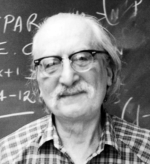
This can be viewed as a matrix question. The action of the i-th student sharing water can be viewed as a linear transformation $A_i$ on the vector of water quantities, indexed by the students. I think that in general the answer to Q1 is “yes.” Here is the Sage code in the case of 3 students:

sage: A1 = matrix(QQ, [[1/3,0,0],[1/3,1,0],[1/3,0,1]])
sage: A2 = matrix(QQ, [[1,1/3,0],[0,1/3,0],[0,1/3,1]])
sage: A3 = matrix(QQ, [[1,0,1/3],[0,1,1/3],[0,0,1/3]])
sage: (A1*A2*A3).eigenvectors_right()                 
[(1, [(1, 2, 3)], 1), 
 (0.1851851851851852? - 0.05237828008789241?*I, 
 [(1, 0.?e-57 + 1.414213562373095?*I, -1.000000000000000? - 1.414213562373095?*I)], 1), 
 (0.1851851851851852? + 0.05237828008789241?*I, 
 [(1, 0.?e-57 - 1.414213562373095?*I, -1.000000000000000? + 1.414213562373095?*I)], 1)]

In other words, the product $A_1A_2A_3$ has eigenvalue $\lambda = 1$ with eigenvector $\vec{v} = (1,2,3)$ . This means that in the case that student 1 has 3 ounces of water, student 2 has 2 ounces of water, student 3 has 1 ounce of water, if each student shares water as explained in the problem, at the end of the process, they will each have the same amount as they started with.

I don’t know the answer to Q2 or Q3.

SymPy and the GSoC

Posted on 2012/04/23 by wdjoyner

Google has announced the results for Google Summer of Code. The following projects have been accepted for SymPy:

(Project, Student, Mentor, Link to proposal on the wiki)
– Category Theory Module, Sergiu Ivanov, Tom Bachmann
– Density Operators for Quantum Module in sympy.physics.quantum, Guru
Devanla, Brian Granger (co-mentor Sean Vig)
– Enhancements to sympy.physics.mechanics, Angadh Nanjangud, Gilbert Gede
– Group Theory, Aleksandar Makelov, David Joyner (Aaron Meurer co-mentor)
– Implicit Plotting Module, Bharath M R, Aaron Meurer
– Vector Analysis, Stefan Krastanov, Matthew Rocklin

I will help mentor Aleksandar Makelov’s work on group theory. He is a freshman at Harvard.

Bifid cipher and Sage

Posted on 2012/01/04 by wdjoyner

The Bifid cipher was invented around 1901 by Felix Delastelle. It is a “fractional substitution” cipher, where letters are replaced by pairs of symbols from a smaller alphabet. The cipher uses a 5×5 square filled with some ordering of the alphabet, except that “i”‘s and “j”‘s are identified (this is a so-called Polybius square; there is a 6×6 analog if you add back in “j” and also append onto the usual 26 letter alphabet, the digits 0, 1, …, 9). According to Helen Gaines’ book “Cryptanalysis”, this type of cipher was used in the field by the German army during World War I.

The Bifid cipher was discusses in Alasdair McAndrew’s book on Cryptography and Sage. We shall follow his discussion. As an example of a Polybius square for the Bifid cipher, pick the key to be “encrypt” (as Alasdair does). In that case, the Polybius square is $\left(\begin{array}{rrrrr} E & N & C & R & Y \\ P & T & A & B & C \\ D & E & F & G & H \\ I & K & L & M & N \\ O & P & Q & R & S \end{array}\right).$ BTW, the $6\times 6$ analog is: $\left(\begin{array}{rrrrrr} E & N & C & R & Y & P \\ T & A & B & C & D & E \\ F & G & H & I & J & K \\ L & M & N & O & P & Q \\ R & S & T & U & V & W \\ X & Y & Z & 0 & 1 & 2 \end{array}\right)$ .

Here is Sage code to produce the $6\times 6$ case (the $5\times 5$ case is in Alasdair’s book):

def bifid(pt, key):
    """
    INPUT:
        pt - plaintext string      (digits okay)
        key - short string for key (no repetitions, digits okay)
    
    OUTPUT:
        ciphertext from Bifid cipher (all caps, no spaces)

    This is the version of the Bifid cipher that uses the 6x6
    Polybius square.

    AUTHOR:
        Alasdair McAndrew

    EXAMPLES:
        sage: key = "encrypt"
        sage: pt = "meet me on monday at 8am"
        sage: bifid(pt, key)
        [[2, 5], [0, 0], [0, 0], [1, 0], [2, 5], [0, 0], [3, 0], 
         [0, 1], [2, 5], [3, 0], [0, 1], [1, 3], [1, 1], [0, 4], 
         [1, 1], [1, 0], [5, 4], [1, 1], [2, 5]]
        'HNHOKNTA5MEPEGNQZYG'

    """
    AS = AlphabeticStrings()
    A = list(AS.alphabet())+[str(x) for x in range(10)]
    # first make sure the letters are capitalized
    # and text has no spaces
    key0 = [x.capitalize() for x in key if not(x.isspace())]
    pt0 = [x.capitalize() for x in pt if not(x.isspace())]
    # create long key
    long_key = key0+[x for x in A if not(x in key0)]
    n = len(pt0)
    # the fractionalization
    pairs = [[long_key.index(x)//6, long_key.index(x)%6] for x in pt0]
    print pairs
    tmp_cipher = flatten([x[0] for x in pairs]+[x[1] for x in pairs])
    ct = join([long_key[6*tmp_cipher[2*i]+tmp_cipher[2*i+1]] for i in range(n)], sep="")
    return ct

def bifid_square(key):
    """
    Produced the Polybius square for the 6x6 Bifid cipher.

    EXAMPLE:
        sage: key = "encrypt"
        sage: bifid_square(key)
        [E N C R Y P]
        [T A B C D E]
        [F G H I J K]
        [L M N O P Q]
        [R S T U V W]
        [X Y Z 0 1 2]

    """
    AS = AlphabeticStrings()
    A = list(AS.alphabet())+[str(x) for x in range(10)]
    # first make sure the letters are capitalized
    # and text has no spaces
    key0 = [SR(x.capitalize()) for x in key if not(x.isspace())]
    # create long key
    long_key = key0+[SR(x) for x in A if not(x in key0)]
    # the fractionalization
    pairs = [[long_key.index(SR(x))//6, long_key.index(SR(x))%6] for x in A]
    f = lambda i,j: long_key[6*i+j] 
    M = matrix(SR, 6, 6, f)
    return M

Have fun!

God’s number for the Rubik’s cube in the face turn metric

Posted on 2010/08/29 by wdjoyner

This is an update to the older post.

The story is described well at cube20.org but the bottom line is that Tom Rokicki, Herbert Kociemba, Morley Davidson, and John Dethridge have established that every cube position can be solved in 20 face moves or less. The superflip is known to take 20 moves exactly (in 1995, Michael Reid established this), so 20 is best possible – or God’s number in the face turn algorithm. Google (and, earlier, Sony) contributed computer resources to do the needed massive computations. Congradulations to everyone who worked on this!

This would make a great documentary I think!

uniform matroids and MDS codes

Posted on 2010/03/10 by wdjoyner

It is known that uniform (resp. paving) matroids correspond to MDS (resp. “almost MDS” codes). This post explains this connection.

An MDS code is an $[n,k,d]$ linear error correcting block code $C$ which meets the Singleton bound, $d+k=n+1$ . A uniform matroid is a matroid for which all circuits are of size $\geq r(M)+1$ , where $r(M)$ is the rank of M. Recall, a circuit in a matroid M=(E,J) is a minimal dependent subset of E — that is, a dependent set whose proper subsets are all independent (i.e., all in J).

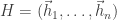
Consider a linear code $C$ whose check matrix is an $(n-k)\times n$ matrix $H=(\vec{h}_1,\dots , \vec{h}_n)$ . The vector matroid M=M[H] is a matroid for which the smallest sized dependency relation among the columns of H is determined by the check relations $c_1\vec{h}_1 + \dots + c_n \vec{h}_n = H\vec{c}=\vec{0}$ , where $\vec{c}=(c_1,\dots,c_n)$ is a codeword (in C which has minimum dimension d). Such a minimum dependency relation of H corresponds to a circuit of M=M[H].

Floyd-Warshall-Roy, 3

Posted on 2010/03/02 by wdjoyner

As in the previous post, let $G=(V,E)$ be a weighted digraph having $n$ vertices and let $A=A_G$ denote its $n\times n$ adjacency matrix. We identify the vertices with the set $\{1,2,\dots, n\}$ .

The previous post discussed the following result, due to Sturmfels et al.

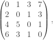
Theorem: The entry of the matrix A^n-1 in row i and column j equals the length of a shortest path from vertex i to vertex j in G. (Here A^n-1 denotes the n-1-st tropical power of A.)

This post discusses an implementation in Python/Sage.

Consider the following class definition.

class TropicalNumbers:
    """
    Implements the tropical semiring.

    EXAMPLES:
        sage: T = TropicalNumbers()
        sage: print T
        Tropical Semiring

    """
    def __init__(self):
        self.identity = Infinity

    def __repr__(self):
        """
        Called to compute the "official" string representation of an object.
        If at all possible, this should look like a valid Python expression
        that could be used to recreate an object with the same value.

        EXAMPLES:
            sage: TropicalNumbers()
            TropicalNumbers()

        """
        return "TropicalNumbers()"

    def __str__(self):
        """
        Called to compute the "informal" string description of an object. 

        EXAMPLES:
            sage: T = TropicalNumbers()
            sage: print T
            Tropical Semiring

        """
        return "Tropical Semiring"

    def __call__(self, a):
        """
        Coerces a into the tropical semiring.

        EXAMPLES:
            sage: T(10)
            TropicalNumber(10)
            sage: print T(10)
            Tropical element 10 in Tropical Semiring
        """
        return TropicalNumber(a)

    def __contains__(self, a):
        """
        Implements "in".

        EXAMPLES:
            sage: T = TropicalNumbers()
            sage: a = T(10)
            sage: a in T
            True

        """
        if a in RR or a == Infinity:
            return a==Infinity or (RR(a) in RR)
        else:
            return a==Infinity or (RR(a.element) in RR)

class TropicalNumber:
    def __init__(self, a):
        self.element = a
        self.base_ring = TropicalNumbers()

    def __repr__(self):
        """
        Called to compute the "official" string representation of an object.
        If at all possible, this should look like a valid Python expression
        that could be used to recreate an object with the same value.

        EXAMPLES:

        """
        return "TropicalNumber(%s)"%self.element

    def __str__(self):
        """
        Called to compute the "informal" string description of an object. 

        EXAMPLES:
            sage: T = TropicalNumbers()
            sage: print T(10)
            Tropical element 10 in Tropical Semiring
        """
        return "%s"%(self.number())

    def number(self):
        return self.element

    def __add__(self, other):
        """
        Implements +. Assumes both self and other are instances of
        TropicalNumber class.

        EXAMPLES:
            sage: T = TropicalNumbers()
            sage: a = T(10)
            sage: a in T
            True
            sage: b = T(15)
            sage: a+b
            10

        """
        T = TropicalNumbers()
        return T(min(self.element,other.element))

    def __mul__(self, other):
        """
        Implements multiplication *.

        EXAMPLES:
            sage: T = TropicalNumbers()
            sage: a = T(10)
            sage: a in T
            True
            sage: b = T(15)
            sage: a*b
            25
        """
        T = TropicalNumbers()
        return T(self.element+other.element)

class TropicalMatrix:
    def __init__(self, A):
        T = TropicalNumbers()
        self.base_ring = T
        self.row_dimen = len(A)
        self.column_dimen = len(A[0])
        # now we coerce the entries into T
        A0 = A
        m = self.row_dimen
        n = self.column_dimen
        for i in range(m):
            for j in range(n):
                A0[i][j] = T(A[i][j])
        self.array = A0

    def matrix(self):
        """
        Returns the entries (as ordinary numbers).

        EXAMPLES:
            sage: A = [[0,1,3,7],[2,0,1,3],[4,5,0,1],[6,3,1,0]]
            sage: AT = TropicalMatrix(A)
            sage: AT.matrix()
            [[0, 1, 3, 7], [2, 0, 1, 3], [4, 5, 0, 1], [6, 3, 1, 0]]
        """
        m = self.row_dim()
        n = self.column_dim()
        A0 = [[0 for i in range(n)] for j in range(m)]
        for i in range(m):
            for j in range(n):
                A0[i][j] = (self.array[i][j]).number()
        return A0

    def row_dim(self):
        return self.row_dimen

    def column_dim(self):
        return self.column_dimen

    def __repr__(self):
        """
        Called to compute the "official" string representation of an object.
        If at all possible, this should look like a valid Python expression
        that could be used to recreate an object with the same value.

        EXAMPLES:

        """
        return "TropicalMatrix(%s)"%self.array

    def __str__(self):
        """
        Called to compute the "informal" string description of an object. 

        EXAMPLES:

        """
        return "Tropical matrix %s"%(self.matrix())

    def __add__(self, other):
        """
        Implements +. Assumes both self and other are instances of
        TropicalMatrix class.

        EXAMPLES:
            sage: A = [[1,2,Infinity],[3,Infinity,0]]
            sage: B = [[2,Infinity,1],[3,-1,1]]
            sage: AT = TropicalMatrix(A)
            sage: BT = TropicalMatrix(B)
            sage: AT
            TropicalMatrix([[TropicalNumber(1), TropicalNumber(2), TropicalNumber(+Infinity)],
              [TropicalNumber(3), TropicalNumber(+Infinity), TropicalNumber(0)]])
            sage: AT+BT
            [[TropicalNumber(1), TropicalNumber(2), TropicalNumber(1)],
             [TropicalNumber(3), TropicalNumber(-1), TropicalNumber(0)]]
        """
        A = self.array
        B = other.array
        C = []
        m = self.row_dim()
        n = self.column_dim()
        if m != other.row_dim:
            raise ValueError, "Row dimensions must be equal."
        if n != other.column_dim:
            raise ValueError, "Column dimensions must be equal."
        for i in range(m):
            row = [A[i][j]+B[i][j] for j in range(n)] # + as tropical numbers
            C.append(row)
        return C

    def __mul__(self, other):
        """
        Implements multiplication *.

        EXAMPLES:
            sage: A = [[1,2,Infinity],[3,Infinity,0]]
            sage: AT = TropicalMatrix(A)
            sage: B = [[2,Infinity],[-1,1],[Infinity,0]]
            sage: BT = TropicalMatrix(B)
            sage: AT*BT
             [[TropicalNumber(1), TropicalNumber(3)],
              [TropicalNumber(5), TropicalNumber(0)]]
            sage: A = [[0,1,3,7],[2,0,1,3],[4,5,0,1],[6,3,1,0]]
            sage: AT = TropicalMatrix(A)
            sage: A = [[0,1,3,7],[2,0,1,3],[4,5,0,1],[6,3,1,0]]
            sage: AT = TropicalMatrix(A)
            sage: print AT*AT*AT
            Tropical matrix [[0, 1, 2, 3], [2, 0, 1, 2], [4, 4, 0, 1], [5, 3, 1, 0]]
        """
        T = TropicalNumbers()
        A = self.matrix()
        B = other.matrix()
        C = []
        mA = self.row_dim()
        nA = self.column_dim()
        mB = other.row_dim()
        nB = other.column_dim()
        if nA != mB:
            raise ValueError, "Column dimension of A and row dimension of B must be equal."
        for i in range(mA):
            row = []
            for j in range(nB):
                c = T(Infinity)
                for k in range(nA):
                    c = c+T(A[i][k])*T(B[k][j])
                row.append(c.number())
            C.append(row)
        return TropicalMatrix(C)

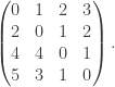
This shows that the shortest distances of digraph with adjacency matrix $\begin{pmatrix} 0&1&3&7\\ 2&0&1&3\\ 4&5&0&1\\ 6&3&1&0\end{pmatrix},$ is equal to A³, which is equal to $\begin{pmatrix} 0&1&2&3\\ 2&0&1&2\\ 4&4&0&1\\ 5&3&1&0\end{pmatrix}.$ This verifies an example given in chapter 1 of the book by Maclagan and Sturmfels, Introduction to Tropical Geometry .

Yet Another Mathblog

Category Archives: software