Introductory example of checking
We may use the field 
It is easy to set up telegraphic codes of high capacity using combinations of four letters each which are not required to be pronounceable. In fact, a sufficiently high capacity may be obtained when only
twenty-three letters of the alphabet are used at all. Hence we can omit any three letters whose Morse equivalents (dot-dash) are most frequently used. Let us suppose that we have before us a code of this kind which employs the letters
and avoids, for reasons stated of for some good reason, the three letters


Suppose that, by prearrangement with telegraphic correspondents, the letters used are paired in
an arbitrary, but fixed, way with the thwenty-three elements of
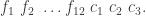
Let the pairings be, for instance:
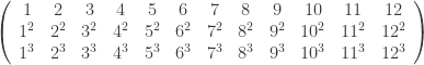
or, in numerical arrangement:


A four-letter group (code word), such as EZRA or XTYP, will indicate a definite entry of a specific page of a definite code volume, several such volumes being perhaps employed in the code. An entry will, in general, be a phrase of sentence, or a group of phrases or sentences, commonly occurring in the class of messages for which the code has been constructed.
Suppose that we have agreed to provide, in our messages, three-letter checks upon groups of twelve letters; in other words, to check in one operation a sequence of three four-letter code words. The twelve letters of the three code words are thus expanded to fifteen; but we send just three telegraphic words — three combinations of five letters, each of which is, in general, unpronounceable.
For illustration, let the first three code words of a message be:
The corresponding sequence of paired elements in

This is our operand sequence 


Let us determine the checking matrix 
Thus the 

or

Referring to the multiplication table of
For the first element 

For the second element 
of the multiplication table, and in that row read: 


For the third element 
of the multiplication table, and in that row read: 


The fifth, eighth, and tenth rows of the table will not be used, since


We have 


We transmit, of course, the sequence of letters paired, in our system of communications, with the elements of the sequence,
Thus we transmit the sequence of letters: XTYP VZRV HVHH RIF; but we may conveniently agree to transmit it in the arrangement:

or in some other arrangement which employs only three telegraphic words (unpronounceable five letter groups).
We could have used other reference matrices, but we shall not stop to discuss this point. We may remark, however, that if the matrix

had been adopted, the checking elements would have been

and their evaluation would have been accomplished with equal
ease by means of the multiplication table of
 identical socks and
  from
from ![[0,1]](https://s0.wp.com/latex.php?latex=%5B0%2C1%5D&bg=ffffff&fg=323232&s=0&c=20201002) randomly until
randomly until  first exceeds
  . What is the probability that this happens on the fourth draw? That is, what is the probability that
  and
and  ?
? that a plane is divided into by
  straight lines in the plane?
 that
that  -dimensional Euclidean space is divided into by
  , the number of regions that are bounded, and for
  , the number of regions that are unbounded.
 Explain why these numbers are correct.
 matrices with random integer entries. (These entries are as likely to be even as to be odd.) Joe, being a bit of a gambler, wants to bet Bob a dollar that the next matrix will have an even determinant. Should Bob take the bet? What is the probability that the next matrix will have an even determinant?
 .
. matrix with randomly chosen integer entries is divisible by the prime number
  ?
? are equally likely for each integer entry.)
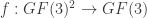 .
. that can be defined as
 . We call
  bent if
 (here
(here  ). Such ternary (or
  -ary) bent functions have been studied by a number of authors. Here we shall only consider those ternary bent functions of two variables which are even (in the sense
  ) and
) and  .
. such functions.
 is shown here (thanks to Sage):
 with
with  vertices, and this is it!


 ),
),
 forms a
  ! In fact,
  .
. ?
? 

 on the vector of water quantities, indexed by the students. I think that in general the answer to Q1 is “yes.” Here is the Sage code in the case of 3 students:
 has eigenvalue
  with eigenvector
  . This means that in the case that student 1 has 3 ounces of water, student 2 has 2 ounces of water, student 3 has 1 ounce of water, if each student shares water as explained in the problem, at the end of the process, they will each have the same amount as they started with.
 is not prime.
 ,
, 

 an arbitrary element of this field, we see that negatives and reciprocals of the elements of the field are as shown in the scheme:


 . By the usual methods, it is quickly found that one solution is (
 ,
,  ,
,  ). The general solution is (
 ,
,  ,
,  denotes an element of the field.
 ,
,  .
.
 . It may be observed in passing that if
 .
. ,
,  ,
, 
 be
be  which we shall call the “affix” of the mark
  is given by the formula
 is the smallest non-negative integer satisfying

 is the smallest non-negative integer satisfying

 elements of our field then


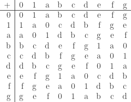
 elements. An addition table is not needed. The multiplication table is as follows:
 are negatives —
  ,
,  — when
  . In the present example, therefore, two marks
  are negatives if
 are momentarily regarded as ordinary integers of familiar arithmetic.
 . We shall use it in illustrating our checking operations.
 , so that we may write


 being irreducible in

 is not the square of an element in
You must be logged in to post a comment.