Lester Hill’s “The checking of the accuracy …”, part 3

Posted on 2012/06/05 by wdjoyner

Backstory: Lester Saunders Hill wrote unpublished notes, about 40 pages long, probably in the mid- to late 1920s. They were titled “The checking of the accuracy of transmittal of telegraphic communications by means of operations in finite algebraic fields”. In the 1960s this manuscript was given to David Kahn by Hill’s widow. The notes were typewritten, but mathematical symbols, tables, insertions, and some footnotes were often handwritten. The manuscript is being LaTeXed “as we speak”. I thank Chris Christensen, the National Cryptologic Museum, and NSA’s David Kahn Collection, for their help in obtaining these notes. Many thanks also to Rene Stein of the NSA Cryptologic Museum library and David Kahn for permission to publish this transcription. Comments by transcriber will look his this: [This is a comment. – wdj]. I used Sage (www.sagemath.org) to generate the tables in LaTeX.

Here is just the third section of his paper. I hope to post more later. (Part 2 is here.)

Section 3: Preliminary characterization of checking procedure

Our problem is to provide convenient and practical accuracy checks upon a sequence of $n$ elements $f_1$ , $f_2$ , $\dots$ , $f_n$ in a finite algebraic field $F$ .

To fix the ideas, let us assume that we are to employ $q$ -element checks $c_1$ , $c_2$ , $\dots$ , $c_q$ upon the sequence $f_1$ , $f_2$ , $\dots$ , $f_n$ . The checks are to be determined by means of a fixed reference matrix

$Q = \left( \begin{array}{cccc} k_{11} & k_{12} & \dots & k_{1n} \\ k_{21} & k_{22} & \dots & k_{2n} \\ \vdots & & & \vdots \\ k_{q1} & k_{q2} & \dots & k_{qn} \\ \end{array} \right)$
of elements of $F$ , the matrix having been suitably constructed according to criteria which will be developed in the following pages. We send, in place of the simple sequence $f_1$ , $f_2$ , $\dots$ , $f_n$ , the amplified sequence

$f_1, f_2, \dots, f_n, c_1, c_2, \dots, c_q$
consisting of the “operand” sequence and the “checking” sequence. The checking sequence contains $q$ elements of $F$ as follows:

$c_j = \sum_{i=1}^n k_{ji}f_i,$

for $j = 1, 2, \dots, q$ . Considerations of telegraphic economy dictate the assumption, made throughout the paper, that $q\leq n$ .

Before laying down specifications for the reference matrix $Q$ , we define a matrix of “index” $q$ as one in which no $q$ -rowed determinant vanishes.

Lester Hill’s “The checking of the accuracy …”, part 2

Posted on 2012/06/03 by wdjoyner

Here is just the second section of his paper. I hope to post more later. (Part 1 is here.)

Secton 2: Lemmas concerning algebraic fields

Familiarity with primary notions in the theory of finite algebraic fields, and of their algebraic extensions, will naturally be assumed here. Reference is made, however, to Steinitz [St], Dickson [D], Scorza [Sc]. But several points which will be needed very frequently in the following pages are summarized here in a series of lemmas. These lemmas assert properties of any algebraic field, whether it be finite or not.

Lemma 1:
Let $F$ denote an algebraic field. Let the coeefficients $a_{ij}$ in the system of equations

$\begin{array}{c} a_{11}x_1 +a_{12}x_2 +\dots + a_{1n}x_n=0\\ a_{21}x_1 +a_{22}x_2 +\dots + a_{2n}x_n=0\\ \vdots \\ a_{n1}x_1 +a_{n2}x_2 +\dots + a_{nn}x_n=0, \\ \end{array}$

be elements of $F$ . Let $\Delta$ denote the value, in $F$ , of the determinant

$\begin{array}{|ccc|} a_{11} & \dots & a_{1n} \\ \vdots && \\ a_{n1} & \dots & a_{nn} \\ \end{array} \, .$
The system of equations has a solution other than

$x_1 = x_2 = \dots = x_n = 0$

if and only if $\Delta =0$ .

Lemma 2:
Let $F$ denote an algebraic field. Let the coeefficients in the system of equations

$\begin{array}{c} a_{11}x_1 +a_{12}x_2 +\dots + a_{1n}x_n=0\\ a_{21}x_1 +a_{22}x_2 +\dots + a_{2n}x_n=0\\ \vdots \\ a_{k1}x_1 +a_{k2}x_2 +\dots + a_{kn}x_n=0, \\ \end{array}$

be elements of $F$ , and let $k$ be less than $n$ . Then the system of equations certainly has a solution other than
$x_1 = x_2 = \dots = x_n = 0\, .$

Lemma 3:
Let $F$ denote an algebraic field. Let the $a_{ij}$ and the $c_i$ denote elements of $F$ and let at least one of the $c_i$ be different from zero. Consider the determinant

$\Delta = \begin{array}{|ccc|} a_{11} & \dots & a_{1n} \\ \vdots && \\ a_{n1} & \dots & a_{nn} \\ \end{array} \, .$
If $\Delta \not=0$ (Footnote: The case $\Delta = 0$ does not concern us.) then the system of equations

$\begin{array}{c} a_{11}x_1 +a_{12}x_2 +\dots + a_{1n}x_n=0\\ a_{21}x_1 +a_{22}x_2 +\dots + a_{2n}x_n=0\\ \vdots \\ a_{n1}x_1 +a_{n2}x_2 +\dots + a_{nn}x_n=0, \\ \end{array}$

has one and only one solution.

Evidently, when solutions exist for the systems of equations considered in the forgoing three lemmas, such solutions lie entirely in the field $F$ .

The lemma which follows is particularly useful. It is an immediate corollary of Lemma 1.

Lemma 4:
Let $F$ denote an algebraic field. Let the $a_{ij}$ denote elements of $F$ . Then if

$\begin{array}{|ccc|} a_{11} & \dots & a_{1n} \\ \vdots && \\ a_{n1} & \dots & a_{nn} \\ \end{array} =0, \, .$

we can determine at least one sequence of elements $\lambda_1$ , $\lambda_2$ , $\dots$ , $\lambda_n$ , which are not necessarily distinct but certainly are not all equal to zero, such that

$\begin{array}{c} a_{11}\lambda_1 +a_{21}\lambda_2 +\dots + a_{n1}\lambda_n=0\\ a_{12}\lambda_1 +a_{22}\lambda_2 +\dots + a_{n2}\lambda_n=0\\ \vdots \\ a_{1n}\lambda_1 +a_{2n}\lambda_2 +\dots + a_{nn}\lambda_n=0. \\ \end{array}$

Lemma 5:
The algebraic equation of $ $n$ th degree

$a_0x^n + a_1 x^{n-1} + \dots + a_{n-1}x+a_n=0,$

with coefficients in the algebraic field $F$ , can not have more than $n$ roots in $F$ .

Most of the considerations of the present paper will depend, more or less directly, upon these five lemmas.

References:

[D] L. E. Dickson, Linear groups with an exposition of the Galois field theory, B. G. Teubner, Leipzig, 1901. Available here:
http://archive.org/details/lineargroupswith00dickuoft

[Sc] G. Scorza, Corpi numerici e algebre, Giuseppe Principato, 1921.

[St] E. Steinitz, Algebraische theorie der korper, Journal fur die reine und angew. Mathamtik 137(1910)167-308.

Lester Hill’s “The checking of the accuracy …”, part 1

Posted on 2012/05/30 by wdjoyner

Backstory: Lester Saunders Hill wrote an unpublished notes, 40 pages, undated but probably written in mid- to late 1920s, titled “The checking of the accuracy of transmittal of telegraphic communications by means of operations in finite algebraic fields”. In the 1960s this was given to David Kahn by Hill’s widow. These notes were typewritten, but mathematical symbols, tables, insertions, and some footnotes were often handwritten. These notes are being LaTeXed “as we speak”. I thank Chris Christensen, the National Cryptologic Museum, and NSA’s David Kahn Collection, for their help in obtaining these notes. Many thanks also to Rene Stein of the NSA Cryptologic Museum library and David Kahn for permission to publish this transcription. Comments by transcriber will look his this: [This is a comment. – wdj]. I used Sage (www.sagemath.org) to generate the tables in LaTeX.

Here is just the introductory first section of his paper. I hope to post more later.

Section 1: The problem considered

The forms of code in current use for the economical transmittal of cable and radio messages employ, almost uniformly, the so-called ”pronounceable” combinations. Pronounceability is estimated in terms of letter groups which commonly occur in one or more of eight designated ”telegraphic” languages: English, French, Spanish, etc. International regulations have, in fact, prescribed a system, of charges according to which a secret five-letter word is regarded, in the word count, as one-half of a telegraphic word, or as a full telegraphic word, according to as it is, or is not, pronounceable.

There is now descernible a definite tendancy to abandon this quite arbitrary pronounceability rule, which has heretofore hampered the development of code and cipher communication. And it seems not unlikely that, at some early session of the Interbational Telegraph Congress, all secret five-letter combinations will be placed upon the same basis with respect to transmittal charges.

A mathematical problem of considerable scientific and practical interest arises in this connection. Messages written in pronounceable code or cipher contain within themselves certain checks upon the accuracy of their telegraphic transmittal. But sequences of unpronounceable groups will generally be quite arbitrary, and no such internal check will ordinarily be available. The outstanding requirement is some device capable of protecting totally unrestricted sequences, in a telegraphically economical way, against the hazards of faulty transmittal.

Let the finite set $C$ of signs (letters, numerals, etc) upon which a given system of communication is based – plain-language, code, or cipher system – be placed in correspondence with the elements of a finite algebraic field $F$ . Then the problem of checking sequences of signs in $C$ becomes that of checking sequences of elements in $F$ . As well-known, if we denote by $\Gamma$ the number of elements, including the zero and unit elements, of a finite field $F$ , then $\Gamma$ is one of the numbers:

$2, 3, 4, 5, 7, 8, 9, 11, 13, 16, 17, 19, 23, 25, 27, 29, 31, 32, \dots ,$

that is to say, $\Gamma$ is of the form $\Gamma = p^r$ , where $p$ denotes a prime positive integer greater than $1$ and $r$ denotes a positive integer. Conversely, if $\Gamma$ is an integer of this form, we can very easily set up finite algebraic fields with $\Gamma$ elements. In devising a scheme of checks for messages based upon the system $C$ of communications with $n$ distinct signs, we should normally work with a field $F$ the number, $\Gamma$ , of whose elements differs as little as possible form $n$ . But this is not essential.

Our problem, viewed form the standpoint of mathematics, is simply that of providing economical and rigorous checks, easily applied in a practical way, upon the accuracy of transmittal of arbitrary sequences of elements in a finite algebraic field.

The method suggested will be applicable to telegraphic messages of any type: plain-language, code, cipher, cipher-code. It will, however, undoubtedly, be found susceptible of fundamental improvement in many respects; and it will probably yield to other, and more definitely practical, procedures that may subsequently be constructed be upon a basis of number-theoretical operations. The present paper will have served its purpose if it succeeds in directing attention to certain hitherto neglected practical possibilites inherent in elementary algebraic manipulations.

SymPy and the GSoC

Posted on 2012/04/23 by wdjoyner

Google has announced the results for Google Summer of Code. The following projects have been accepted for SymPy:

(Project, Student, Mentor, Link to proposal on the wiki)
– Category Theory Module, Sergiu Ivanov, Tom Bachmann
– Density Operators for Quantum Module in sympy.physics.quantum, Guru
Devanla, Brian Granger (co-mentor Sean Vig)
– Enhancements to sympy.physics.mechanics, Angadh Nanjangud, Gilbert Gede
– Group Theory, Aleksandar Makelov, David Joyner (Aaron Meurer co-mentor)
– Implicit Plotting Module, Bharath M R, Aaron Meurer
– Vector Analysis, Stefan Krastanov, Matthew Rocklin

I will help mentor Aleksandar Makelov’s work on group theory. He is a freshman at Harvard.

A remark on mathematical research

Posted on 2012/04/21 by wdjoyner

Ira Glass, of This American Life (http://www.thisamericanlife.org/), did an excellent four-part interview where he talked at length about writing news stories. They are here:

Ira Glass on Storytelling:
part 1 of 4 http://www.youtube.com/watch?v=loxJ3FtCJJA&feature=relmfu
part 2 of 4 http://www.youtube.com/watch?v=KW6x7lOIsPE&feature=fvwrel
part 3 of 4 http://www.youtube.com/watch?v=BI23U7U2aUY&feature=fvwrel
part 4 of 4 http://www.youtube.com/watch?v=baCJFAGEuJM&feature=relmfu

I thought a lot of what he said was based on general principles which applied to mathematical research as well. Here is perhaps what he would have said if he was talking about mathematics, sometimes with direct quotes from his interview:

There are two building blocks to a idea for a paper

The problem or question. This is sometimes an issue in the intersection of two fields or a question of why some object of interest behaves the way you think it does, based on an example you know.
The revelation. This might be a key example or technique that will hopefully reveal the answer to your question.

You can have a great question, but if they don’t turn out to have any useful techniques or examples to work with, your idea is uninteresting. Conversely you can have a significant revelation with a fantastically powerful method, but if the problem or examples themselves are uninteresting, again you’ve got a weak idea.

You have to set aside just as much time looking for good ideas as you do producing them. In other words, the work of thinking up a good idea to write about is as much work and time as writing it up.

Not enough gets said about the importance of abandoning crap. Most of your story ideas are going to be crap. That’s okay because the only way you can surface great ideas is by going through a lot of crappy ones. The only reason you want to be doing this is to make something memorable and special.

“The thing I’d like to say to you with all my heart is that most everybody I know who does interesting creative work went through a phase of years where with their good taste, they could tell what they were doing wasn’t as good as they wanted it to be … it didn’t have that special thing they wanted it to have … Everybody goes through that phase … and the most important thing you can do is do a lot of work.”

Sestinas and Sage

Posted on 2012/04/02 by wdjoyner

According to [1], a sestina is a highly structured poem consisting of six six-line stanzas followed by a tercet (called its envoy or tornada), for a total of thirty-nine lines. The same set of six words ends the lines of each of the six-line stanzas, but in a shuffled order each time. The shuffle used is very similar to the Mongean shuffle.

Define $f_n(k) = 2k$ , if k <= n/2 and $f_n(k) = 2n+1-2k$ , if $k > n/2.$ Let $p = (p_1,...,p_n) \in S_n$ , where $p_j = f_n(p_{j-1})$ and $S_n$ is the symmetric group of order $n$ . From [2], we have the following result.

Theorem: If p is an n-cycle then 2n+1 is a prime.

Call such a prime a “sestina prime”. Which primes are sestina primes?

Here is Python/Sage code for this permutation:


def sestina(n):
    """
    Computes the element of the symmetric group S_n associated to the shuffle above. 
  
    EXAMPLES: 
        sage: sestina(4)
        (1,2,4) 
        sage: sestina(6)
        (1,2,4,5,3,6)
        sage: sestina(8)
        (1,2,4,8)(3,6,5,7)
        sage: sestina(10)
        (1,2,4,8,5,10)(3,6,9)
        sage: sestina(12)
        (1,2,4,8,9,7,11,3,6,12)(5,10)
        sage: sestina(14)
        (1,2,4,8,13,3,6,12,5,10,9,11,7,14) 
        sage: sestina(16)
        (1,2,4,8,16)(3,6,12,9,15)(5,10,13,7,14)
        sage: sestina(18)
        (1,2,4,8,16,5,10,17,3,6,12,13,11,15,7,14,9,18)
        sage: sestina(20) (1,2,4,8,16,9,18,5,10,20)(3,6,12,17,7,14,13,15,11,19) 
        sage: sestina(22) (1,2,4,8,16,13,19,7,14,17,11,22)(3,6,12,21)(5,10,20)(9,18) 

    """ 
    def fcn(k, n):
        if k<=int(n/2): 
            return 2*k 
        else: 
            return 2*n+1-2*k 
    L = [fcn(k,n) for k in range(1,n+1)] 
    G = SymmetricGroup(n) 
    return G(L)

And here is an example due to Ezra Pound [3]:

                                  I

Damn it all! all this our South stinks peace.
You whoreson dog, Papiols, come! Let’s to music!
I have no life save when the swords clash.
But ah! when I see the standards gold, vair, purple, opposing
And the broad fields beneath them turn crimson,
Then howl I my heart nigh mad with rejoicing.

                                     II

In hot summer have I great rejoicing
When the tempests kill the earth’s foul peace,
And the light’nings from black heav’n flash crimson,
And the fierce thunders roar me their music
And the winds shriek through the clouds mad, opposing,
And through all the riven skies God’s swords clash.

                                     III

Hell grant soon we hear again the swords clash!
And the shrill neighs of destriers in battle rejoicing,
Spiked breast to spiked breast opposing!
Better one hour’s stour than a year’s peace
With fat boards, bawds, wine and frail music!
Bah! there’s no wine like the blood’s crimson!

                                     IV

And I love to see the sun rise blood-crimson.
And I watch his spears through the dark clash
And it fills all my heart with rejoicing
And prys wide my mouth with fast music
When I see him so scorn and defy peace,
His lone might ’gainst all darkness opposing.

                                     V

The man who fears war and squats opposing
My words for stour, hath no blood of crimson
But is fit only to rot in womanish peace
Far from where worth’s won and the swords clash
For the death of such sluts I go rejoicing;
Yea, I fill all the air with my music.

                                     VI

Papiols, Papiols, to the music!
There’s no sound like to swords swords opposing,
No cry like the battle’s rejoicing
When our elbows and swords drip the crimson
And our charges ’gainst “The Leopard’s” rush clash.
May God damn for ever all who cry “Peace!”

                                     VII

And let the music of the swords make them crimson
Hell grant soon we hear again the swords clash!
Hell blot black for always the thought “Peace”!

References:

[1] http://en.wikipedia.org/wiki/Sestina

[2] Richard Dore and Anton Geraschenko,”Sestinas and Primes” posted to http://stacky.net/wiki/index.php?title=Course_notes, and http://math.berkeley.edu/~anton/written/sestina.pdf

[3] Ezra Pound, “Sestina: Altaforte” (1909), (originally published int the English Review, 1909)

[4] John Bullitt, N. J. A. Sloane and J. H. Conway , http://oeis.org/A019567

Remarks on the Hamming [7.4.3] code and Sage

Posted on 2012/02/28 by wdjoyner

This post simply collects some very well-known facts and observations in one place, since I was having a hard time locating a convenient reference.

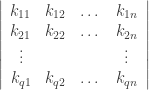
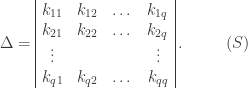
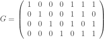
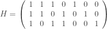
Let $C$ be the binary Hamming [7,4,3] code defined by the generator matrix $G = \left(\begin{array}{rrrrrrr} 1 & 0 & 0 & 0 & 1 & 1 & 1 \\ 0 & 1 & 0 & 0 & 1 & 1 & 0 \\ 0 & 0 & 1 & 0 & 1 & 0 & 1 \\ 0 & 0 & 0 & 1 & 0 & 1 & 1 \end{array}\right)$ and check matrix $H = \left(\begin{array}{rrrrrrr} 1 & 1 & 1 & 0 & 1 & 0 & 0 \\ 1 & 1 & 0 & 1 & 0 & 1 & 0 \\ 1 & 0 & 1 & 1 & 0 & 0 & 1 \end{array}\right)$ . In other words, this code is the row space of G and the kernel of H. We can enter these into Sage as follows:

sage: G = matrix(GF(2), [[1,0,0,0,1,1,1],[0,1,0,0,1,1,0],[0,0,1,0,1,0,1],[0,0,0,1,0,1,1]])
sage: G
[1 0 0 0 1 1 1]
[0 1 0 0 1 1 0]
[0 0 1 0 1 0 1]
[0 0 0 1 0 1 1]
sage: H = matrix(GF(2), [[1,1,1,0,1,0,0],[1,1,0,1,0,1,0],[1,0,1,1,0,0,1]])
sage: H
[1 1 1 0 1 0 0]
[1 1 0 1 0 1 0]
[1 0 1 1 0 0 1]
sage: C = LinearCode(G)
sage: C
Linear code of length 7, dimension 4 over Finite Field of size 2
sage: C = LinearCodeFromCheckMatrix(H)
sage: LinearCode(G) == LinearCodeFromCheckMatrix(H)
True

The generator matrix gives us a one-to-one onto map $G:GF(2)^4\to C$ defined by $m \longmapsto m\cdot G$ . Using this map, the codewords are easy to describe and enumerate:

$\begin{tabular}{ccc} decimal & binary & codeword \\ 0 & 0000 & 0000000 \\ 1 & 0001 & 0001011 \\ 2 & 0010 & 0010101 \\ 3 & 0011 & 0011110 \\ 4 & 0100 & 0100110 \\ 5 & 0101 & 0101101 \\ 6 & 0110 & 0110011 \\ 7 & 0111 & 0111000 \\ 8 & 1000 & 1000111 \\ 9 & 1001 & 1001100 \\ 10 & 1010 & 1010010 \\ 11 & 1011 & 1011001 \\ 12 & 1100 & 1100001 \\ 13 & 1101 & 1101010 \\ 14 & 1110 & 1110100 \\ 15 & 1111 & 1111111 \end{tabular}$ .

Using this code, we first describe a guessing game you can play with even small children.

Number Guessing game: Pick an integer from 0 to 15. I will ask you 7 yes/no questions. You may lie once.
I will tell you when you lied and what the correct number is.

Question 1: Is n in {0,1,2,3,4,5,6,7}?
(Translated: Is 1st bit of Hamming_code(n) a 0?)
Question 2: Is n in {0,1,2,3,8,9,10,11}?
(Is 2nd bit of Hamming_code(n) a 0?)
Question 3: Is n in {0,1,4,5,8,9,12,13}?
(Is 3rd bit of Hamming_code(n) a 0?)
Question 4: Is n in {0,2,4,6,8,10,12,14} (ie, is n even)?
(Is 4th bit of Hamming_code(n) a 0?)
Question 5: Is n in {0,1,6,7,10,11,12,13}?
(Is 5th bit of Hamming_code(n) a 0?)
Question 6: Is n in {0,2,5,7,9,11,12,14}?
(Is 6th bit of Hamming_code(n) a 0?)
Question 7: Is n in {0,3,4,7,9,10,13,14}?
(Is 7th bit of Hamming_code(n) a 0?)

Record the answers in a vector (0 for yes, 1 for no): $v = (v_1,v_2,...,v_7)$ . This must be a codeword (no lies) or differ from a codeword by exactly one bit (1 lie). In either case, you can find n by decoding this vector.

We discuss a few decoding algorithms next.

Venn diagram decoding:

We use a simple Venn diagram to describe a decoding method.

sage: t = var('t')
sage: circle1 = parametric_plot([10*cos(t)-5,10*sin(t)+5], (t,0,2*pi))
sage: circle2 = parametric_plot([10*cos(t)+5,10*sin(t)+5], (t,0,2*pi))
sage: circle3 = parametric_plot([10*cos(t),10*sin(t)-5], (t,0,2*pi))
sage: text1 = text("$1$", (0,0))  
sage: text2 = text("$2$", (-6,-2)) 
sage: text3 = text("$3$", (0,7))
sage: text4 = text("$4$", (6,-2)) 
sage: text5 = text("$5$", (-9,9)) 
sage: text6 = text("$6$", (9,9)) 
sage: text7 = text("$7$", (0,-9))  
sage: textA = text("$A$", (-13,13)) 
sage: textB = text("$B$", (13,13)) 
sage: textC = text("$C$", (0,-17)) 
sage: text_all = text1+text2+text3+text4+text5+text6+text7+textA+textB+textC
sage: show(circle1+circle2+circle3+text_all,axes=false)

This gives us the following diagram:

Decoding algorithm:
Suppose you receive $v = ( v_1, v_2, v_3, v_4, v_5, v_6, v_7)$ .
Assume at most one error is made.
Decoding process:

Place $v_i$ in region i of the Venn diagram.
For each of the circles A, B, C, determine if the sum of the bits in four regions add up to 0 or to 1. If they add to 1, say that that circle has a “parity failure”.
The error region is determined form the following table.

$\begin{tabular}{cc} parity failure region(s) & error position \\ none & none \\ A, B, and C & 1 \\ B, C & 4 \\ A, C & 2 \\ A, B & 3 \\ A & 5 \\ B & 6 \\ C & 7 \end{tabular}$

For example, suppose v = (1,1,1,1,1,0,1). The filled in diagram looks like

This only fails in circle B, so the table says (correctly) that the error is in the 6th bit. The decoded codeword is $c = v+e_6 = (1,1,1,1,1,1,1).$

Next, we discuss a decoding method based on the Tanner graph.

Tanner graph for hamming 7,4,3 code

The above Venn diagram corresponds to a bipartite graph, where the left “bit vertices” (1,2,3,4,5,6,7) correspond to the coordinates in the codeword and the right “check vertices” (8,9,10) correspond to the parity check equations as defined by the check matrix. This graph corresponds to the above Venn diagram, where the check vertices 8, 9, 10 were represented by circles A, B, C:

sage: Gamma = Graph({8:[1,2,3,5], 9:[1,2,4,6], 10:[1,3,4,7]})
sage: B = BipartiteGraph(Gamma)
sage: B.show()
sage: B.left
set([1, 2, 3, 4, 5, 6, 7])
sage: B.right
set([8, 9, 10])
sage: B.show()

This gives us the graph in the following picture:

Decoding algorithm:
Suppose you receive $v = ( v_1, v_2, v_3, v_4, v_5, v_6, v_7)$ .
Assume at most one error is made.
Decoding process:

Place $v_i$ at the vertex i on the left side of the bipartite graph.
For each of the check vertices 8,9,10 on the right side of the graph, determine of the if the sum of the bits in the four left-hand vertices connected to it add up to 0 or to 1. If they add to 1, we say that that check vertex has a “parity failure”.
Those check vertices which do not fail are connected to bit vertices which we assume are correct. The remaining bit vertices
connected to check vertices which fail are to be determined (if possible) by solving the corresponding check equations.

check vertex 8: $v_2+v_3+v_4+v_5 = 0$

check vertex 9: $v_1+v_3+v_4+v_6 = 0$

check vertex 10: $v_1+v_2+v_4+v_7 = 0$

Warning: This method is not guaranteed to succeed in general. However, it does work very efficiently when the check matrix H is “sparse” and the number of 1’s in each row and column is “small.”

For example, suppose v = (1,1,1,1,1,0,1). The check vertex 9 fails its parity check, but vertex 8 and 10 do not. Therefore, only bit vertex 6 is unknown, since vertex 6 is the only one not connected to 8 and 10. This tells us that the decoding codeword is $c = (1,1,1,1,1,v_6,1)$ , for some unknown $v_6$ . We solve for this unknown using the check vertex equation $v_1+v_3+v_4+v_6 = 0$ , giving us $v_6 = 1$ . The decoded codeword is $c = (1,1,1,1,1,1,1).$

This last example was pretty simple, so let’s try $v=(0,1,1,1,1,1,1)$ . In this case, we know the vertices 9 and 10 fail, so $c = (v_1,1,1,1,1,v_6,v_7)$ . We solve using

$v_1+1+1+v_6 = 0$

$v_1+1+1+v_7 = 0$

This simply tells us $v_1=v_6=v_7$ . By majority vote, we get $c = (1,1,1,1,1,1,1)$ .

Digital steganography and Sage

Posted on 2012/02/22 by wdjoyner

This post shall explain how the F5 stegosystem (in a simple case) can be implemented in Sage. I thank Carlos Munuera for teaching me these ideas and for many helpful conversations on this matter. I also thank Kyle Tucker-Davis [1] for many interesting conversations on this topic.

Steganography, meaning “covered writing,” is the science of secret communication [4]. The medium used to carry the information is called the “cover” or “stego-cover” (depending on the context – these are not synonymous terms). The term “digital steganography” refers to secret communication where the cover is a digital media file.

One of the most common systems of digital steganography is the Least Significant Bit (LSB) system. In this system, we assume the “cover” image is represented as a finite sequence of binary vectors of a given length. In other words, a greyscale image is regarded as an array of pixels, where each pixel is represented by a binary vector of a certain fixed length. Each such vector represents a pixel’s brightness in the cover image. The encoder embeds (at most) one bit of information in the least significant bit of eaach vector. Care must be taken with this system to ensure that the changes made do not betray the stego-cover, while still maximizing the information hidden.

From a short note of Crandell [3] in 1998, it was realized that error-correcting codes can give rise to “stego-schemes”, ie, methods by which a message can be hidden in a digital file efficiently.

Idea in a nutshell: If $C$ is the r-th binary Hamming code (so, $n = 2^r-1$ is its length, $k = 2^r - r - 1$ is its dimension, and $d = 3$ is its minimum distance), $G$ is a generating matrix, $H$ is a check matrix, and $C^\perp$ is the dual code of $C$ , then we take an element $v \in GF(2)^n$ to be a cover, and the message $m$ we embed is an element of $GF(2)^r$ . Once we find a vector $z$ of lowest weight such that $H(v+z)=m$ , we call $v+z$ the stegocover. The stegocover looks a lot like the original cover and “contains” the message m. This will be explained in more detai below.
(This particular scheme is called the F5 stegosystem, and is due to Westfeld.)

Quick background on error-correcting, linear, block codes [5]

A linear error-correcting block code is a finite dimensional vector space over a finite field with a fixed basis. We assume the finite field is the binary field $GF(2)$ .

We shall typically think of a such a code as a subspace $C$ of $GF(2)^n$ with a fixed basis, where $n>0$ is an integer called the length of the code. Moreover, the basis for the ambient space $GF(2)^n$ will be the standard basis,

$e_1=(1,0,\dots, 0), e_2=(0,1,0,\dots, 0), \dots, e_n=(0,\dots, 0,1).$

There are two common ways to specify a linear code $C$ .

You can give $C$ as a vector subspace of $GF(2)^n$ by specifying a set of basis vectors for $C$ . This set of basis vectors is, by convention, placed as
the rows of a matrix called a generator matrix $G$ of $C$ . Obviously, the order in which the rows are presented does not
affect the code itself.

If $g_1, \dots, g_k$ are the rows of $G$ then

$C= \{c=m_1g_1+\dots +m_kg_k\ |\ {\rm some}\ m_i\in GF(2)\},$

is the set of linear combinations of the row vectors $g_i$ . The vector of coefficients, $m=(m_1,\dots, m_k)$ represents the information you want to encode and transmit.

In other words, encoding of a message can be defined via the generator matrix:

$\begin{array}{ccc} m = (m_1,\dots, m_k) & \to & c=m_1g_1+\dots +m_kg_k = m^t\cdot G,\\ GF(2)^k & \to & C. \end{array}$
You can give $C$ as a vector subspace of $GF(2)^n$ by specifying a matrix $H$ for which $C$ is the kernel of $H$ , $C={\rm ker}(C)$ . This matrix is called a check matrix of $C$ . Again, the order in which the rows are presented does not affect the code itself.

Note that if $G$ is a full rank $k\times n$ matrix then a full rank check matrix $H$ must be a $(n-k) \times n$ matrix.

These two ways of defining a code are not unrelated.

Fact:
If $G=(I_k\ \vert\ A)$ is the generating matrix for $C$ then $H=(-A^t\ \vert\ I_{n-k})$ is a parity check matrix.

Exaample:
Let $r>0$ be an integer and let $H$ be a $r\times (2^r-1)$ matrix whose columns are all the distinct non-zero vectors of $GF(2)^r$ . Then, the code having $H$ as its check matrix is called a binary Hamming code, denoted Ham(r,2).

Let $r=3$ , and let

$H= \begin{pmatrix} 0 & 1 & 1 & 1 & 1 & 0 & 0 \\ 1 & 0 & 1 & 1 & 0 & 1 & 0 \\ 1 & 1 & 0 & 1 & 0 & 0 & 1 \end{pmatrix}.$

In this form, namely when the columns of $H$ are arranged in standard form such that the rightmost $k\times k$ entries is the identity matrix $I_k$ , the generator matrix $G$ can be quickly found to be

$G= \begin{pmatrix} 1 & 0 & 0 & 0 & 0 & 1 & 1 \\ 0 & 1 & 0 & 0 & 1 & 0 & 1 \\ 0 & 0 & 1 & 0 & 1 & 1 & 0 \\ 0 & 0 & 0 & 1 & 1 & 1 & 1 \end{pmatrix}.$

A coset of $GF(2)^n/C$ is a subset of $GF(2)^n$ of the form $C+v$ for some $v\in GF(2)^n$ . Let $S$ be a coset of $C$ . Then,
a coset leader of $S$ is an element of $S$ having smallest Hamming weight.

Fact:
The coset leaders of a Hamming code are those vectors of $wt \leq 1$ .

Steganographic systems from error-correcting codes

This section basically describes Crandell’s idea [3] in a more formalized language.

Following Munuera’s notation in [6], a steganographic system $S$ can be formally defined as

$S= \{\mathcal{C}, \mathcal{M}, \mathcal{K}, emb, rec \},$
where

$\mathcal{C}$ is a set of all possible covers
$\mathcal{M}$ is a set of all possible messages
$\mathcal{K}$ is a set of all possible keys
$emb:\mathcal{C}\times\mathcal{M}\times\mathcal{K}\to\mathcal{C}$ is an embedding function
$rec:\mathcal{C}\times\mathcal{K}\to\mathcal{M}$ is a recovery function

and these all satisfy

$rec(emb(c,m,k),k)=m,$

for all $m\in\mathcal{M}$ , $c\in\mathcal{C}$ , $k\in\mathcal{K}$ . We will assume that a fixed key $k\in\mathcal{K}$ is used, and therefore,
the dependence on an element in the keyspace $\mathcal{K}$ can be ignored. The original cover $c$ is called the plain cover, $m$ is called the message, and $emb(c,m,k)=emb(c,m)$ is called the stegocover. Let $\mathcal{C}$ be $GF(2)^n$ , representing both plain covers and stegocovers. Also, let $\mathcal{M}$ be $GF(2)^k$ , where $k$ is a fixed integer such that $0 \leq k \leq n$ .

Sage examples

How do we compute the emb map?

We need the following Sage function.

def hamming_code_coset_leader(C, y):
      """
      Finds the coset leader of a binary Hamming code C.
      EXAMPLES:
      """
      F = C.base_ring()
      n = C.length()
      k = C.dimension()
      r = n-k
      V0 = F^r
      if not(y in V0):
          RaiseError, "Input vector is not a syndrome."
      H = C.check_mat()
      colsH = H.columns()
      i = colsH.index(y)
      V = F^n
      v = V(0)
      v[i] = F(1)
      return v

Let $V = GF(2)^{63}$ and consider the cover $v = ([1,1,1,1,1,1,1,1,1,1,1,1,1,1,1,1,1,1, 1,1,1,1,0,0,1,1,1, 1,0,0,0,0,0,0,1,1,1,0,0,0,0,0,0,0,1,1,0,0,0,0,0,0,1,1,1,0,0,1,1,0,0,1,1)$ . Regarded as a $7\times 9$ matrix,

V = GF(2)^(63)
rhino = V([1,1,1,1,1,1,1,1,1,
           1,1,1,1,1,1,1,1,1,
           1,1,1,1,0,0,1,1,1,
           1,0,0,0,0,0,0,1,1,
           1,0,0,0,0,0,0,0,1,
           1,0,0,0,0,0,0,1,1,
           1,0,0,1,1,0,0,1,1])
A = matrix(GF(2),7,rhino.list())
matrix_plot(A)

this looks like an elephant or a rhino:

Now we embed the message $m = (1,0,1,0,1,0)$ . First we compute the stegocover:

C = HammingCode(6,GF(2))
H = C.check_mat()
V0 = GF(2)^6
m = V0([1,0,1,0,1,0])
z = hamming_code_coset_leader(C, m)
stegocover = rhino+z
A = matrix(GF(2),7,stegocover.list())
matrix_plot(A)

It looks like another rhino/elephant:

Note only one bit is changed since the Hamming weight of z is at most 1. To recover the message m, just multiply the vector “stegocover” by H.

That’s how you can use Sage to understand the F5 stegosystem, at least in a very simple case.

REFERENCES:
[1] Kyle Tucker-Davis, “An analysis of the F5 steganographic system”, Honors Project 2010-2011
http://www.usna.edu/Users/math/wdj/tucker-davis/

[2] J. Bierbrauer and J. Fridrich. “Constructing good covering codes for applications in Steganography}. 2006.
http://www.math.mtu.edu/jbierbra/.

[3] Crandall, Ron. “Some Notes on Steganography”. Posted on a Steganography Mailing List, 1998.
http://os.inf.tu-dresden.de/westfeld/crandall.pdf

[4] Wayner, Peter. Disappearing Cryptography. Morgan Kauffman Publishers. 2009.

[5] Hill, Raymond. A First Course in Coding Theory. Oxford University Press. 1997.

[6] Munuera, Carlos. “Steganography from a Coding Theory Point of View”. 2010.
http://www.singacom.uva.es/oldsite/Actividad/s3cm/s3cm10/10courses.html

[7] Zhang, Weiming and S. Li. “Steganographic Codes- a New Problem of Coding Theory”. preprint, 2005.
http://arxiv.org/abs/cs/0505072.

Applications of graphs to Boolean functions

Posted on 2012/02/16 by wdjoyner

Let f be a Boolean function on $GF(2)^n$ . The Cayley graph of f is defined to be the graph

$\Gamma_f = (GF(2)^n, E_f )$ ,

whose vertex set is $GF(2)^n$ and the set of edges is defined by

$E_f =\{ (u,v) \in GF(2)^n \times GF(2)^n \ |\ f(u+v)=1\}$ .

The adjacency matrix $A_f$ is the matrix whose entries are

$A_{i,j} = f(b(i) + b(j))$ ,

where b(k) is the binary representation of the integer k.
Note $\Gamma_f$ is a regular graph of degree wt(f), where wt denotes the Hamming weight of f when regarded as a vector of values (of length $2^n$ ).

Recall that, given a graph $\Gamma$ and its adjacency matrix A, the spectrum Spec( $\Gamma$ ) is the multi-set of eigenvalues of A.

The Walsh transform of a Boolean function f is an integer-valued function over $GF(2)^n$ that can be defined as

$W_f(u) = \sum_{x in GF(2)^n} (-1)^{f(x)+ \langle u,x\rangle}.$
A Boolean function f is bent if $|W_f(a)| = 2^{n/2}$ (this only makes sense if n is even). The Hadamard transform of a integer-valued function f is an integer-valued function over $GF(2)^n$ that can be defined as

$H_f(u) = \sum_{x in GF(2)^n} f(x)(-1)^{\langle u,x\rangle}.$
It turns out that the spectrum of $\Gamma_f$ is equal to the Hadamard transform of f when regarded as a vector of (integer) 0,1-values. (This nice fact seems to have first appeared in [2], [3].)

A graph is regular of degree r (or r-regular) if every vertex has degree r (number of edges incident to it).   We say that an r-regular graph $\Gamma$ is a strongly regular graph with parameters (v, r, d, e) (for nonnegative integers e, d) provided, for all vertices u, v the number of vertices adjacent to both u, v is equal to

          e, if u, v are adjacent,
          d, if u, v are nonadjacent.

It turns out tht f is bent iff $\Gamma_f$ is strongly regular and e = d (see [3] and [4]).

The following Sage computations illustrate these and other theorems in [1], [2], [3], [4].

Consider the Boolean function $f: GF(2)^4 \to GF(2)$ given by $f(x_0,x_1,x_2) = x_0x_1+x_2x_3$ .

sage: V = GF(2)^4
sage: f = lambda x: x[0]*x[1]+x[2]*x[3]
sage: CartesianProduct(range(16), range(16))
Cartesian product of [0, 1, 2, 3, 4, 5, 6, 7, 8, 9, 10, 11, 12, 13, 14, 15], 
                     [0, 1, 2, 3, 4, 5, 6, 7, 8, 9, 10, 11, 12, 13, 14, 15]
sage: C = CartesianProduct(range(16), range(16))
sage: Vlist = V.list()                  
sage: E = [(x[0],x[1]) for x in C if f(Vlist[x[0]]+Vlist[x[1]])==1]
sage: len(E)
96
sage: E = Set([Set(s) for s in E])
sage: E = [tuple(s) for s in E] 
sage: Gamma = Graph(E)
sage: Gamma
Graph on 16 vertices
sage: VG = Gamma.vertices()
sage: L1 = []
sage: L2 = []
sage: for v1 in VG:
....:         for v2 in VG:
....:             N1 = Gamma.neighbors(v1)
....:         N2 = Gamma.neighbors(v2)
....:         if v1 in N2:
....:                 L1 = L1+[len([x for x in N1 if x in N2])]
....:         if not(v1 in N2) and v1!=v2:
....:                 L2 = L2+[len([x for x in N1 if x in N2])]
....: 
....: 
sage: L1; L2
[2, 2, 2, 2, 2, 2, 2, 2, 2, 2, 2, 2, 2, 2, 2, 2, 2, 2, 2, 2,
 2, 2, 2, 2, 2, 2, 2, 2, 2, 2, 2, 2, 2, 2, 2, 2, 2, 2, 2, 2,
 2, 2, 2, 2, 2, 2, 2, 2, 2, 2, 2, 2, 2, 2, 2, 2, 2, 2, 2, 2,
 2, 2, 2, 2, 2, 2, 2, 2, 2, 2, 2, 2, 2, 2, 2, 2, 2, 2, 2, 2,
 2, 2, 2, 2, 2, 2, 2, 2, 2, 2, 2, 2, 2, 2, 2, 2]
[2, 2, 2, 2, 2, 2, 2, 2, 2, 2, 2, 2, 2, 2, 2, 2, 2, 2, 2, 2,
 2, 2, 2, 2, 2, 2, 2, 2, 2, 2, 2, 2, 2, 2, 2, 2, 2, 2, 2, 2,
 2, 2, 2, 2, 2, 2, 2, 2, 2, 2, 2, 2, 2, 2, 2, 2, 2, 2, 2, 2,
 2, 2, 2, 2, 2, 2, 2, 2, 2, 2, 2, 2, 2, 2, 2, 2, 2, 2, 2, 2,
 2, 2, 2, 2, 2, 2, 2, 2, 2, 2, 2, 2, 2, 2, 2, 2, 2, 2, 2, 2,
 2, 2, 2, 2, 2, 2, 2, 2, 2, 2, 2, 2, 2, 2, 2, 2, 2, 2, 2, 2,
 2, 2, 2, 2, 2, 2, 2, 2, 2, 2, 2, 2, 2, 2, 2, 2, 2, 2, 2, 2,
 2, 2, 2, 2]

This implies the graph is strongly regular with d=e=2.

sage: Gamma.spectrum()
[6, 2, 2, 2, 2, 2, 2, -2, -2, -2, -2, -2, -2, -2, -2, -2]
sage: [walsh_transform(f, a) for a in V]
[4, 4, 4, -4, 4, 4, 4, -4, 4, 4, 4, -4, -4, -4, -4, 4]
sage: Omega_f = [v for v in V if f(v)==1] 
sage: len(Omega_f)
6
sage: Gamma.is_bipartite()
False
sage: Gamma.is_hamiltonian()
True
sage: Gamma.is_planar()     
False
sage: Gamma.is_regular()
True
sage: Gamma.is_eulerian()
True
sage: Gamma.is_connected()
True
sage: Gamma.is_triangle_free()
False
sage: Gamma.diameter()
2
sage: Gamma.degree_sequence()
[6, 6, 6, 6, 6, 6, 6, 6, 6, 6, 6, 6, 6, 6, 6, 6]
sage: show(Gamma)
# bent-fcns-cayley-graphs1.png

Here is the picture of the graph:

sage: H = matrix(QQ, 16, 16, [(-1)^(Vlist[x[0]]).dot_product(Vlist[x[1]]) for x in C])
sage: H
[ 1  1  1  1  1  1  1  1  1  1  1  1  1  1  1  1]
[ 1 -1  1 -1  1 -1  1 -1  1 -1  1 -1  1 -1  1 -1]
[ 1  1 -1 -1  1  1 -1 -1  1  1 -1 -1  1  1 -1 -1]
[ 1 -1 -1  1  1 -1 -1  1  1 -1 -1  1  1 -1 -1  1]
[ 1  1  1  1 -1 -1 -1 -1  1  1  1  1 -1 -1 -1 -1]
[ 1 -1  1 -1 -1  1 -1  1  1 -1  1 -1 -1  1 -1  1]
[ 1  1 -1 -1 -1 -1  1  1  1  1 -1 -1 -1 -1  1  1]
[ 1 -1 -1  1 -1  1  1 -1  1 -1 -1  1 -1  1  1 -1]
[ 1  1  1  1  1  1  1  1 -1 -1 -1 -1 -1 -1 -1 -1]
[ 1 -1  1 -1  1 -1  1 -1 -1  1 -1  1 -1  1 -1  1]
[ 1  1 -1 -1  1  1 -1 -1 -1 -1  1  1 -1 -1  1  1]
[ 1 -1 -1  1  1 -1 -1  1 -1  1  1 -1 -1  1  1 -1]
[ 1  1  1  1 -1 -1 -1 -1 -1 -1 -1 -1  1  1  1  1]
[ 1 -1  1 -1 -1  1 -1  1 -1  1 -1  1  1 -1  1 -1]
[ 1  1 -1 -1 -1 -1  1  1 -1 -1  1  1  1  1 -1 -1]
[ 1 -1 -1  1 -1  1  1 -1 -1  1  1 -1  1 -1 -1  1]
sage: flist = vector(QQ, [int(f(v)) for v in V])
sage: H*flist  
(6, -2, -2, 2, -2, -2, -2, 2, -2, -2, -2, 2, 2, 2, 2, -2)
sage: A = matrix(QQ, 16, 16, [f(Vlist[x[0]]+Vlist[x[1]]) for x in C])
sage: A.eigenvalues()
[6, 2, 2, 2, 2, 2, 2, -2, -2, -2, -2, -2, -2, -2, -2, -2]

Here is another example: $f: GF(2)^3 \to GF(2)$ given by $f(x_0,x_1,x_2) = x_0x_1+x_2$ .

sage: V = GF(2)^3
sage: f = lambda x: x[0]*x[1]+x[2]
sage: Omega_f = [v for v in V if f(v)==1] 
sage: len(Omega_f)
4
sage: C = CartesianProduct(range(8), range(8))
sage: Vlist = V.list()    
sage: E = [(x[0],x[1]) for x in C if f(Vlist[x[0]]+Vlist[x[1]])==1]
sage: E = Set([Set(s) for s in E])
sage: E = [tuple(s) for s in E] 
sage: Gamma = Graph(E)
sage: Gamma
Graph on 8 vertices
sage: 
sage: VG = Gamma.vertices()
sage: L1 = []
sage: L2 = []
sage: for v1 in VG:
....:         for v2 in VG:
....:             N1 = Gamma.neighbors(v1)
....:         N2 = Gamma.neighbors(v2)
....:         if v1 in N2:
....:                 L1 = L1+[len([x for x in N1 if x in N2])]
....:         if not(v1 in N2) and v1!=v2:
....:                 L2 = L2+[len([x for x in N1 if x in N2])]
....: 
sage: L1; L2
[2, 0, 2, 2, 2, 2, 0, 2, 2, 2, 0, 2, 2, 2, 2, 0, 0, 2, 2, 2, 2, 0, 2, 2, 2, 0, 2, 2, 2, 2, 0, 2]
[2, 2, 2, 2, 2, 2, 2, 2, 2, 2, 2, 2, 2, 2, 2, 2, 2, 2, 2, 2, 2, 2, 2, 2]

This implies that the graph is not strongly regular, therefore f is not bent.

sage: Gamma.spectrum()
[4, 2, 0, 0, 0, -2, -2, -2]
sage: 
sage: Gamma.is_bipartite()
False
sage: Gamma.is_hamiltonian()
True
sage: Gamma.is_planar()     
False
sage: Gamma.is_regular()
True
sage: Gamma.is_eulerian()
True
sage: Gamma.is_connected()
True
sage: Gamma.is_triangle_free()
False
sage: Gamma.diameter()
2
sage: Gamma.degree_sequence()
[4, 4, 4, 4, 4, 4, 4, 4]
sage: H = matrix(QQ, 8, 8, [(-1)^(Vlist[x[0]]).dot_product(Vlist[x[1]]) for x in C])
sage: H
[ 1  1  1  1  1  1  1  1]
[ 1 -1  1 -1  1 -1  1 -1]
[ 1  1 -1 -1  1  1 -1 -1]
[ 1 -1 -1  1  1 -1 -1  1]
[ 1  1  1  1 -1 -1 -1 -1]
[ 1 -1  1 -1 -1  1 -1  1]
[ 1  1 -1 -1 -1 -1  1  1]
[ 1 -1 -1  1 -1  1  1 -1]
sage: flist = vector(QQ, [int(f(v)) for v in V])
sage: H*flist  
(4, 0, 0, 0, -2, -2, -2, 2)
sage: Gamma.spectrum()
[4, 2, 0, 0, 0, -2, -2, -2]
sage: A = matrix(QQ, 8, 8, [f(Vlist[x[0]]+Vlist[x[1]]) for x in C])
sage: A.eigenvalues()
[4, 2, 0, 0, 0, -2, -2, -2]

sage: show(Gamma)
# bent-fcns-cayley-graphs2.png

Here is the picture:

REFERENCES:
[1] Pantelimon Stanica, Graph eigenvalues and Walsh spectrum of Boolean functions, INTEGERS 7(2) (2007), #A32.

[2] Anna Bernasconi, Mathematical techniques for the analysis of Boolean functions, Ph. D. dissertation TD-2/98, Universit di Pisa-Udine, 1998.

[3] Anna Bernasconi and Bruno Codenotti, Spectral Analysis of Boolean Functions as a Graph Eigenvalue Problem, IEEE TRANSACTIONS ON COMPUTERS, VOL. 48, NO. 3, MARCH 1999.

[4] A. Bernasconi, B. Codenotti, J.M. VanderKam. A Characterization of Bent Functions in terms of Strongly Regular Graphs, IEEE Transactions on Computers, 50:9 (2001), 984-985.

[5] Michel Mitton, Minimal polynomial of Cayley graph adjacency matrix for Boolean functions, preprint, 2007.

[6] ——, On the Walsh-Fourier analysis of Boolean functions, preprint, 2006.

The Vigenère cipher and Sage

Posted on 2012/01/20 by wdjoyner

The Vigenère cipher is named after Blaise de Vigenère, a sixteenth century diplomat and cryptographer, by a historical accident. Vigene`re actually invented a different and more complicated cipher. The so-called “Vigenère cipher” cipher was actually invented by Giovan Batista Belaso in 1553. In any case, it is this cipher which we shall discuss here first.

This cipher has been re-invented by several authors, such as author and mathematician Charles Lutwidge Dodgson (Lewis Carroll) who claimed his 1868 “The Alphabet Cipher” was unbreakable. Several others claimed the so-called Vigenère cipher was unbreakable (e.g., the Scientific American magazine in 1917). However, Friedrich Kasiski and Charles Babbage broke the cipher in the 1800’s [1]. This cipher was used in the 1700’s, for example, during the American Civil War. The Confederacy used a brass cipher disk to implement the Vigenère cipher (now on display in the NSA Museum in Fort Meade) [1].

The so-called Vigenère cipher is a generalization of the Cesaer shift cipher. Whereas the shift cipher shifts each letter by the same amount (that amount being the key of the shift cipher) the so-called Vigenère cipher shifts a letter by an amount determined by the key, which is a word or phrase known only to the sender and receiver).

For example, if the key was a single letter, such as “C”, then the so-called Vigenère cipher is actually a shift cipher with a shift of 2 (since “C” is the 2-nd letter of the alphabet, if you start counting at 0). If the key was a word with two letters, such as “CA”, then the so-called Vigenère cipher will shift letters in even positions by 2 and letters in odd positions are left alone (or shifted by 0, since “A” is the 0-th letter, if you start counting at 0).

REFERENCES:
[1] Wikipedia article on the Vigenere cipher.

Using Sage, let’s look at a message (a chant at football games between rivals USNA and West Point):

sage: AS = AlphabeticStrings()           
sage: A = AS.alphabet()
sage: VC = VigenereCryptosystem(AS, 1) # sets the key length to be = 1
sage: m = VC.encoding("Beat Army!"); m  # trivial example
BEATARMY

Now, we choose for illustration a simple key of length 1, and encipher this message:

sage: key = AS("D")
sage: c = VC.enciphering(key, m)
sage: c  # a trivial example
EHDWDUPB

You see here that in this case the cipher boils down to the Caesar/shift cipher (shifting by 3).

Deciphering is easy:

sage: VC.deciphering(key, c)
BEATARMY

Next, we choose for illustration a simple key of length 2, and encipher the same message:

sage: VC = VigenereCryptosystem(AS, 2)
sage: key = AS("CA")
sage: m = VC.encoding("Beat Army!"); m
BEATARMY
sage: c = VC.enciphering(key, m); c
DECTCROY

Since one of the key letters is “A” (which shifts by 0), half the plaintext is unchanged in going to the ciphertext.

Here is the algorithmic description of the above (so-called) Vigenère cipher:

    ALGORITHM:
    INPUT: 
      key - a string of upper-case letters (the secret "key")
      m - string of upper-case letters (the "plaintext" message)
    OUTPUT:
      c - string of upper-case letters (the "ciphertext" message)

  Identify the alphabet A, ..., Z with the integers 0, ..., 25. 
    Step 1: Compute from the string key a list L1 of corresponding
            integers. Let n1 = len(L1).
    Step 2: Compute from the string m a list L2 of corresponding
            integers. Let n2 = len(L2).
    Step 3: Break L2 up sequencially into sublists of size n1, and one sublist
            at the end of size <=n1. 
    Step 4: For each of these sublists L of L2, compute a new list C given by 
            C[i] = L[i]+L1[i] (mod 26) to the i-th element in the sublist, 
            for each i.
    Step 5: Assemble these lists C by concatenation into a new list of length n2.
    Step 6: Compute from the new list a string c of corresponding letters.

Once it is known that the key is, say, n characters long, frequency analysis can be applied to every n-th letter of the ciphertext to determine the plaintext. This method is called “Kasiski examination“, or the “Kasiski attack” (although it was first discovered by Charles Babbage).

The cipher Vigenère actually discovered is an “auto-key cipher” described as follows.

ALGORITHM:
    INPUT: 
      key - a string of upper-case letters (the secret "key")
      m - string of upper-case letters (the "plaintext" message)
    OUTPUT:
      c - string of upper-case letters (the "ciphertext" message)

  Identify the alphabet A, ..., Z with the integers 0, ..., 25. 
    Step 1: Compute from the string m a list L2 of corresponding
            integers. Let n2 = len(L2). 
    Step 2: Let n1 be the length of the key. Concatenate the string 
            key with the first n2-n1 characters of the plaintext message.
            Compute from this string of length n2 a list L1 of corresponding
            integers. Note n2 = len(L1).
    Step 3: Compute a new list C given by C[i] = L1[i]+L2[i] (mod 26), for each i.
            Note n2 = len(C).
    Step 5: Compute from the new list a string c of corresponding letters.

Note how the key is mixed with the plaintext to create the enciphering of the plaintext to ciphertext in Steps 2 and 3.

A screencast describing this has been posted to vimeo.