Mathematicians and Chess

Posted on 2012/11/12 by wdjoyner

This page contains information on

which mathematicians (which we define as someone who has earned a PhD or equivalent in Mathematics) play(ed) chess at the International Master level or above (in OTB or correspondence or problem composing), and
how to get papers on mathematical chess problems.

Similar pages are here and here and here and here.

Mathematicians who play(ed) chess

Conel Hugh O’Donel Alexander (1909-1974), late British chess champion. Alexander may not have had a PhD in mathematics but taught mathematics and he did mathematical work during WWII (code and cryptography), as did the famous Soviet chess player David Bronstein (see the book Kahn, Kahn on codes). He was the strongest English player after WWII, until Jonathan Penrose appeared.
Adolf Anderssen (1818-1879). Pre World Championships but is regarded as the strongest player in the world between 1859 and 1866. He received a degree (probably not a PhD) in mathematics from Breslau University and taught mathematics at the Friedrichs gymnasium from 1847 to 1879. He was promoted to Professor in 1865 and was given an honorary doctorate by Breslau (for his accomplishments in chess) in 1865.
Magdy Amin Assem (195?-1996) specialized in p-adic representation theory and harmonic analysis on p-adic reductive groups. He published several important papers before a ruptured aneurysm tragically took his life. He was IM strength (rated 2379) in 1996.
Gedeon Barcza (1911-1986), pronounced bartsa, was a Hungarian professor of mathematics and a chess grandmaster. The opening 1.Nf3 d5 2.g3 is called the Barcza System. The opening 1.e4 e6 2.d4 c5 is known as the Barcza-Larsen Defense.
Ludwig Erdmann Bledow (1795-1846) was a German professor of mathematics (PhD). He founded the first German chess association, Berliner Schachgesellschaft, in 1827. He was the first person to suggest an international chess tournament (in a letter to von der Lasa in 1843). His chess rating is not known but he did at one point win a match against Adolf Anderssen.
Robert Coveyou (1915 – 1996) completed an M.S. degree in Mathematics, and joined the Oak Ridge National Laboratory as a research mathematician. He became a recognized expert in pseudo-random number generators. He is known for the quotation “The generation of random numbers is too important to be left to chance,” which is based on a title of a paper he wrote. An excellent tournament chess player, he was Tennessee State Champion eight times.
Nathan Divinsky (1925-2012) earned a PhD in Mathematics in 1950 from the University of Chicago and was a mathematics professor at the University of British Columbia in Vancouver. He tied for first place in the 1959 Manitoba Open.
Noam Elkies (1966-), a Professor of Mathematics at Harvard University specializing in number theory, is a study composer and problem solver (ex-world champion). Prof. Elkies, at age 26, became the youngest scholar ever to have attained a tenured professorship at Harvard. One of his endgame studies is mentioned, for example, in the book Technique for the tournament player, by GM Yusupov and IM Dvoretsky, Henry Holt, 1995. He wrote 11 very interesting columns on Endgame Exporations (posted by permission).
Some other retrograde chess constructions of his may be found at the interesting Dead Reckoning web site of Andrew Buchanan.
See also Professor Elkies’s very interesting Chess and Mathematics Seminar pages.
Thomas Ernst earned a Ph.D. in mathematics from Uppsala Univ. in 2002 and does research in algebraic combinatorics with applications to mathematical physics. His chess rating is about 2400 (FIDE).
Machgielis (Max) Euwe (1901-1981), World Chess Champion from 1935-1937, President of FIDE (Fédération Internationale des Echecs) from 1970 to 1978, and arbitrator over the turbulent Fischer – Spassky World Championship match in Reykjavik, Iceland in 1972. I don’t know as many details of his mathematical career as I’d like. One source gives: PhD (or actually its Dutch equivalent) in Mathematics from Amsterdam University in 1926. Another gives: Doctorate in philosophy in 1923 and taught as a career. Published an important paper on the mathematics of chess “Mengentheoretische Betrachtungen uber das Schachspiel”. This paper lead to a rule change in chess regarding the 3-times repetition draw.
Ed Formanek (194?-), International Master. Ph.D. Rice University 1970. Retired from the mathematics faculty at Penn State Univ. Worked primarily in matrix theory and representation theory.
Stephen L. Jones is an attorney in LA, but when younger, taught math in the UMass system and spent a term as a member of the Institute for Advanced Study in Princeton NJ. He is one rung below the level of International Master at over the board chess; in correspondence chess, he has earned two of the three norms needed to become a Grandmaster.
Charles Kalme (1939-2002), earned his master title in chess at 15, was US Junior champ in 1954, 1955, US Intercollegiate champ in 1957, and drew in his game against Bobby Fischer in the 1960 US championship. In 1960, he also was selected to be on the First Team All-Ivy Men’s Soccer team, as well as the US Student Olympiad chess team. (Incidently, it is reported that this team, which included William Lombary on board one, did so well against the Soviets in their match that Boris Spassky, board one on the Soviet team, was denied forieng travel for two years as punishment.) In 1961 graduated 1st in his class at the Moore School of Electrical Engineering, The University of Pennsylvania, in Philadelphia. He also received the Cane award (a leadership award) that year. After getting his PhD from NYU (advisor Lipman Bers) in 1967 he to UC Berkeley for 2 years then to USC for 4-5 years. He published 2 papers in mathematics in this period, “A note on the connectivity of components of Kleinian groups”, Trans. Amer. Math. Soc. 137 1969 301–307, and “Remarks on a paper by Lipman Bers”, Ann. of Math. (2) 91 1970 601–606. He also translated Siegel and Moser, Lectures on celestial mechanics, Springer-Verlag, New York, 1971, from the German original. He was important in the early stages of computer chess programming. In fact, his picture and annotations of a game were featured in the article “An advice-taking chess computer” which appeared in the June 1973 issue of Scientific American. He was an associate editor at Math Reviews from 1975-1977 and then worked in the computer industry. Later in his life he worked on trying to bring computers to elementary schools in his native Latvia A National Strategy for Bringing Computer Literacy to Latvian Schools. His highest chess rating was acheived later in his life during a “chess comeback”: 2458.
Here is his game against Bobby Fischer referred to above:[Event “?”]
[Site “New York ch-US”]
[Date “1960.??.??”]
[Round “3”]
[White “Fischer, Robert J”]
[Black “Kalme, Charles”]
[Result “1/2-1/2”]
[NIC “”]
[Eco “C92”]
[Opening “Ruy Lopez, Closed, Ragozin-Petrosian (Keres) Variation”]
1.e4 e5 2.Nf3 Nc6 3.Bb5 a6 4.Ba4 Nf6 5.O-O Be7 6.Re1 b5 7.Bb3 O-O 8.c3 d6 9.h3 Nd7 10.a4 Nc5 11.Bd5 Bb7 12.axb5 axb5 13.Rxa8 Qxa8 14.d4 Nd7 15.Na3 b4 16.Nc4 exd4 17.cxd4 Nf6 18.Bg5 Qd8 19.Qa4 Qa8 20.Qxa8 Rxa8 21.Bxf6 Bxf6 22.e5 dxe5 23.Ncxe5 Nxe5 24.Bxb7 Nd3 25.Bxa8 Nxe1 26.Be4 b3 27.Nd2 1/2-1/2
Miroslav Katetov (1918 -1995) earned his PhD from Charles Univ in 1939. Katetov was IM chess player (earned in 1951) and published about 70 research papers, mostly from topology and functional analysis.
Martin Kreuzer (1962-), CC Grandmaster, is rated over 2600 in correspondence chess (ICCF, as of Jan 2000). His OTB rating is over 2300. His specialty is computational commutative algebra and applications. Here is a recent game of his:
Kreuzer, M – Stickler, A
[Eco “B42”]
[Opening “Sicilian, Kan”]
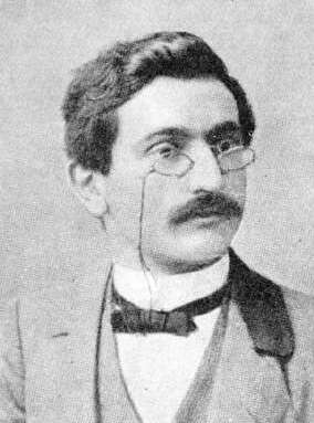
1.e4 c5 2.Nf3 e6 3.d4 cxd4 4.Nxd4 a6 5.Bd3 Nc6 6.c3 Nge7 7.0-0 Ng6 8.Be3 Qc7 9.Nxc6 bxc6 10.f4 Be7 11.Qe2 0-0 12.Nd2 d5 13.g3 c5 14.Nf3 Bb7 15.exd5 exd5 16.Rae1 Rfe8 17.f5 Nf8 18.Qf2 Nd7 19.g4 f6 20.g5 fxg5 21.Nxg5 Bf6 22.Bf4 Qc6 23.Re6 Rxe6 24.fxe6 Bxg5 25.Bxg5 d4 26.Qf7+ Kh8 27.Rf3 Qd5 28.exd7 Qxg5+ 29.Rg3 Qe5 30.d8=Q+ Rxd8 31.Qxb7 Rf8 32.Qe4 Qh5 33.Qe2 Qh6 34.cxd4 cxd4 35.Bxa6 Qc1+ 36.Kg2 Qc6+ 37.Rf3 Re8 38.Qf1 Re3 39.Be2 h6 40.Kf2 Re8 41.Bd3 Qd6 42.Kg1 Kg8 43.a3 Qe7 44.b4 Ra8 45.Qc1 Qd7 46.Qf4 1-0
Emanuel Lasker (1868-1941), World Chess Champion from 1894-1921, PhD (or more precisely its German equivalent) in Mathematics from Erlangen Univ in 1902. Author of the influential paper “Zur theorie der moduln und ideale,” Math. Ann. 60(1905)20-116, where the well-known Lasker-Noether Primary Ideal Decomposition Theorem in Commutative Algebra was proven (it can be downloaded for free here). Lasker wrote and published numerous books and papers on mathematics, chess (and other games), and philosophy.
Vania Mascioni, former IECG Chairperson (IECG is the Internet Email Chess Group), is rated 2326 by IECG (as of 4-99). His area is Functional Analysis and Operator Theory.
A. Jonathan Mestel, grandmaster in over-the-board play and in chess problem solving, is an applied mathematician specializing in fluid mechanics and is the author of numerous research papers. He is on the mathematics faculty of the Imperial College in London.
Walter D. Morris (196?-), International Master. Currently on the mathematics faculty at George Mason Univ in Virginia.
Karsten Müller earned the Grandmaster title in 1998 and a PhD in mathematics in 2002 at the University of Hamburg.
John Nunn (1955-), Chess Grandmaster, D. Phil. (from Oxford Univ.) in 1978 at the age of 23. His PhD thesis is in algebraic topology. Nunn is also a GM chess problem solver.
Hans-Peter Rehm (1942-), earned his PhD in Mathematics from Karlsruhe Univ. (1970) then taught there for many years. He is a grandmaster of chess composition. He has written several papers in mathematics, such as “Prime factorization of integral Cayley octaves”, Ann. Fac. Sci. Toulouse Math (1993), but most in differential algebra, his specialty. A collection of his problems has been published as: Hans+Peter+Rehm=Schach Ausgewählte Schachkompositionen & Aufsätze (= selected chess problems and articles), Aachen 1994.
Kenneth W. Regan, Professor of Computer Science at the State Univ. of New York Buffalo, is currently rated 2453. His research is in computational complexity, a field of computer science which has a significant mathematical component.
Jakob Rosanes obtained his mathematics doctorate from the Univ. of Breslau in 1865 where he taught for the rest of his life. In the 1860s he played a match against A. Anderssen which ended with 3 wins, 3 losses, and 1 draw.
Jan Rusinek (1950-) obtained his mathematics PhD in 1978 and earned a Grandmaster of Chess Composition in 1992.
Jon Speelman (1956-) is an English Grandmaster chess player and chess writer. He earned his PhD in mathematics from Oxford.

Others that might go on this list would be Henry Ernest Atkins (he taught mathematics but never got a PhD, but won the British Chess Championship 9 times in the early 1900s), Andrew Kalotay (who earned a PhD in statistics in 1968 from the Univ of Toronto, and was a Master level chess player but was not formally given an IM chess ranking), Kenneth Rogoff (has a PhD in economics but has published statistics research papers and is a GM in chess), and Duncan Suttles (in the 1960s he started but never finished his PhD in mathematics, but is a chess GM).

Papers about mathematical problems in chess

Timothy Chow, “A Short Proof of the Rook Reciprocity Theorem”, in volume 3, 1996, of the Electronic Journal of Combinatorics.
Noam Elkies, “On numbers and endgames: Combinatorial game theory in chess endgames”, in 1996 “Games of No Chance” = Proceedings of the workshop on combinatorial games held July’94 at MSRI. Available from MSRI Publications — Volume 29 or Noam Elkies’ site.
Noam Elkies and Richard Stanley, “Chess and Mathematics” book (in preparation).
Awani Kumar, “Knight’s Tours in 3 Dimensions”, in The Games and Puzzles Journal The On-line Journal for Mathematical Recreations, Issue 43, January-April 2006.
Richard M. Low and Mark Stamp, “King and Rook Vs. King on a Quarter-Infinite Board“, in Integers, volume 6(2006).
Igor Rivin, Ilan Vardi, Paul Zimmermann, “The N-queens problem“, American Mathematical Monthly 101 (1994), no. 7, 629-639.
Lewis Benjamin Stiller, “Exploiting symmetries on parallel architecture”, PhD thesis, CS Dept, Johns Hopkins Univ. 1995 Closely related is his Games of No Chance paper, “Multilinear Algebra and Chess Endgames“.
Mario VELUCCHI’s math chess problems
Wikipedia’s, Eight queens puzzle.
Herbert S. Wilf, “The Problem of the Kings”, and Michael Larsen, “The Problem of Kings”, both in volume 2, 1995, of the Electronic Journal of Combinatorics.
Papers on odd king tours by D. Joyner and M. Fourte (appeared in the J. of Rec. Math., 2003) and even king tours by M. Kidwell and C. Bailey (in Mathematics Magazine, vol 58, 1985).
Lesson 3 in the chess lessons by Coach Epshteyn at UMBC.

Thanks to Christoph Bandelow, Max Burkett, Elaine Griffith, Hannu Lehto, John Kalme, Ewart Shaw, Richard Stanley, Will Traves, Steven Dowd, Z. Kornin, Noam Elkies and Hal Bogner for help and corrections on this page. This page is an updated version of that page and the other page.

A water sharing problem and Sage

Posted on 2012/10/18 by wdjoyner

Here is the problem: There are n students, each with a cup that could contain water or could be empty. We assume that the cups have no limit and that there is at least one student with some water. Order the students from those who have the most water to those who have the least, with arbitrary choices in cases of ties. Following this order, each student takes turn sharing his water equally with the other students. In other words, a student with r ounces of water will give r/n ounces to each of the others (and hence have r/n ounces remaining for himself).

Q1: Is it possible that there is an initial configuration so that, at the end, all the students have exactly the same amount they started with?
This would mean that sharing was in fact not a loss.

Q2: Will this process “usually even out” the distribution of water?
(Part of the answer is to try to make this question more precise!)

Q3: Does the initial ordering of the students (ie, who pours when) matter?

This can be viewed as a matrix question. The action of the i-th student sharing water can be viewed as a linear transformation $A_i$ on the vector of water quantities, indexed by the students. I think that in general the answer to Q1 is “yes.” Here is the Sage code in the case of 3 students:

sage: A1 = matrix(QQ, [[1/3,0,0],[1/3,1,0],[1/3,0,1]])
sage: A2 = matrix(QQ, [[1,1/3,0],[0,1/3,0],[0,1/3,1]])
sage: A3 = matrix(QQ, [[1,0,1/3],[0,1,1/3],[0,0,1/3]])
sage: (A1*A2*A3).eigenvectors_right()                 
[(1, [(1, 2, 3)], 1), 
 (0.1851851851851852? - 0.05237828008789241?*I, 
 [(1, 0.?e-57 + 1.414213562373095?*I, -1.000000000000000? - 1.414213562373095?*I)], 1), 
 (0.1851851851851852? + 0.05237828008789241?*I, 
 [(1, 0.?e-57 - 1.414213562373095?*I, -1.000000000000000? + 1.414213562373095?*I)], 1)]

In other words, the product $A_1A_2A_3$ has eigenvalue $\lambda = 1$ with eigenvector $\vec{v} = (1,2,3)$ . This means that in the case that student 1 has 3 ounces of water, student 2 has 2 ounces of water, student 3 has 1 ounce of water, if each student shares water as explained in the problem, at the end of the process, they will each have the same amount as they started with.

I don’t know the answer to Q2 or Q3.

Lester Hill’s “The checking of the accuracy …”, part 8

Posted on 2012/10/06 by wdjoyner

Backstory: Lester Saunders Hill wrote unpublished notes, about 40 pages long, probably in the mid- to late 1920s. They were titled “The checking of the accuracy of transmittal of telegraphic communications by means of operations in finite algebraic fields”. In the 1960s this manuscript was given to David Kahn by Hill’s widow. The notes were typewritten, but mathematical symbols, tables, insertions, and some footnotes were often handwritten. I thank Chris Christensen, the National Cryptologic Museum, and NSA’s David Kahn Collection, for their help in obtaining these notes. Many thanks also to Rene Stein of the NSA Cryptologic Museum library and David Kahn for permission to publish this transcription. Comments by transcriber will look like this: [This is a comment. – wdj]. I used Sage (www.sagemath.org) to generate the tables in LaTeX.

Here is just the eighth section of his paper. I hope to post more later. (Part 7 is here.)

Section 8: Examples of finite fields

The reader is probably accustomed to the congruence notation in dealing with finite fields. It may therefore be helpful to insert here two simple examples of finite fields, and to employ, in these concrete cases, the notations of the present paper rather than those of ordinary number theory.

Example: A small field in which the number $\Gamma$ is not prime.

Let the elements of the field be the symbols or marks

$0, 1, a,b,c,d,e,f,g;$
and let us define, by means of two appended tables, the field of operations of addition and multiplcation in such a manner that the marks $0$ , $1$ represent respectively the zero and the unit elements of the field.

These tables are

$\begin{tabular}{r|*{9}{r}} \multicolumn{1}{c|} +&0&1&a&b&c&d&e&f&g\\\hline {}0&0&1&a&b&c&d&e&f&g\\ {}1&1&a&0&c&d&b&f&g&e\\ {}a&a&0&1&d&b&c&g&e&f\\ {}b&b&c&d&e&f&g&1&a&0\\ {}c&c&d&b&f&g&e&a&0&1\\ {}d&d&b&c&g&e&f&0&1&a\\ {}e&e&f&g&1&a&0&c&d&b\\ {}f&f&g&e&a&0&1&d&b&c\\ {}g&g&e&f&0&1&a&b&c&d\\ \end{tabular}$

$\begin{tabular}{r|*{9}{r}} \multicolumn{1}{c|} {*}&0&1&a&b&c&d&e&f&g\\\hline {}0&0&0&0&0&0&0&0&0&0\\ {}1&0&1&a&b&c&d&e&f&g\\ {}a&0&a&1&e&g&f&b&d&c\\ {}b&0&b&e&a&d&g&1&c&f\\ {}c&0&c&g&d&e&1&f&a&b\\ {}d&0&d&f&g&1&b&c&e&a\\ {}e&0&e&b&1&f&c&a&g&d\\ {}f&0&f &d&c&a&e&g&b&1\\ {}g&0&g&c&f&b&a&d&1&e\\ \end{tabular}$

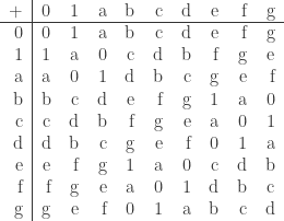
Denoting by $x$ an arbitrary element of this field, we see that negatives and reciprocals of the elements of the field are as shown in the scheme:

$\begin{tabular}{r|rrrrrrrrr} x & 0&1&a&b&c&d&e&f&g\\ \hline -x &0&a&1&e&g&f&b&d&c\\ \hline 1/x & - &1&a&e&d&c&b&g&f \\ \end{tabular}$

The use of notations is easily illustrated. Thus, for example, we note that the determinant

$\Delta = \left| \begin{array}{ccc} f & b & g \\ 1 & f & a \\ d & e & 1 \\ \end{array} \right| \, .$
of the system of equations

$\begin{array}{r} fx+by+gz = 0\\ x+fy+az=0\\ dx+ey+z=0 \end{array}$
vanishes. For, expanding the determinant by the elements of its first row, we obtain

$\begin{array}{lcr} \Delta &= & f(f-ea) - b(1-da)+g(e-fd) \\ &= & f(f+e)+e(1+d)+g(e+b) \\ &= & fc+eb+g(0) =fc+eb=a+1 = 0. \end{array}$
Hence the system has solutions other than $x=y=z=0$ . By the usual methods, it is quickly found that one solution is ( $x=d$ , $y=1$ , $z=0$ ). The general solution is ( $x=\lambda d$ , $y=\lambda$ , $z=0$ ), where $\lambda$ denotes an element of the field.

For further practice, we note that the system of equations

$\begin{array}{rl} bx+gy &= d\\ ax+ez & = 0\\ ex+fy+az &= f \\ \end{array}$
has exactly one solution. It may be found by the standard method employing quotients of determinants [What we call today Cramer’s rule – wdj.]. or as follows:

[11 lines of hand calculations are omitted. – wdj]

The solution is $x=y=f$ , $z=c$ .
$\Box$

As noted in Section 1, the number $\Gamma$ of the elements of a finite algebraic field is either a prime integer greater than $1$ , or a positive integral power of such an integer. In the present example, we have $\Gamma = 9= 3^2$ . It may be observed in passing that if $\lambda$ is any element of a finite field for which

$\Gamma = 2^n,\ \ \ \ \ n\geq 1,$
that is, for which $\Gamma$ is a power of $2$ , then in that field $\lambda = -\lambda$ .

Example: A small field in which the number $\Gamma$ of elements is prime.

Let $f_0$ , $f_1$ , $\dots$ $f_{p-1}$ be $p$ symbols or marks, and let $p$ be a prime integer. We readily define a finite algebraic field of which the elements are the $f_i$ . To this end, we regard $f_i$ as associated with the integer $i$ which we shall call the “affix” of the mark $f_i$ . Understanding that of course $0$ is the “smallest integer” in any set of non-negative integers which includes $0$ , we now define as follows:

Sum: The sum of the marks $f_i$ and $f_j$ is given by the formula

$f_i+f_j = f_k,$
where $k$ is the smallest non-negative integer satisfying

$i+j\equiv k \pmod{p}.$

Product: The product of the marks $f_i$ and $f_j$ is given by the formula

$f_if_j = f_h,$
where $h$ is the smallest non-negative integer satisfying

$ij\equiv h \pmod{p}.$

With the operations of addition and multiplication thus defined, our set of $p$ marks constitutes, as is well-known, an algebraic field. We call a field of this type a “primary” field.
$\Box$

In a primary field, an addition table would never be required. For we note that, if

$f_{j_1}, f_{j_2}, \dots, f_{j_t},$
are $t$ elements of our field then

$\sum_{i=1}^t f_{j_i} = f_k,$
where $k$ is the smallest non-negative integer satisfying the congruence

$\sum_{i=1}^t j_i \equiv k\ \pmod{p}\ .$

Naturally, a similar statement holds for the product. We have

$\prod_{i=1}^t f_{j_i} = f_h,$
where $h$ is the smallest non-negative integer satisfying the congruence

$\prod_{i=1}^t j_i \equiv h\ \pmod{p}\ .$

In the foregoing definitions, any of the terms of a sum, or of the factors of a product, may, of course, be equal.

When dealing with a primary field, we may obviously replace the marks of the fields by their affixes. We do this in the example which follows.

Example: Let the marks of a finite field be

$0,1,2,\dots, 21, 22,$
the field containing $p=23$ elements. An addition table is not needed. The multiplication table is as follows:

$\begin{tabular}{l|rrrrrrrrrrrrrrrrrrrrrr} \ & 1 & 2 & 3 & 4 & 5 & 6 & 7 & 8 & 9 & 10 & 11 & 12 & 13 & 14 & 15 & 16 & 17 & 18 & 19 & 20 & 21 & 22 \\ \hline 1 & 1 & 2 & 3 & 4 & 5 & 6 & 7 & 8 & 9 & 10 & 11 & 12 & 13 & 14 & 15 & 16 & 17 & 18 & 19 & 20 & 21 & 22 \\ 2 & 2 & 4 & 6 & 8 & 10 & 12 & 14 & 16 & 18 & 20 & 22 & 1 & 3 & 5 & 7 & 9 & 11 & 13 & 15 & 17 & 19 & 21 \\ 3 & 3 & 6 & 9 & 12 & 15 & 18 & 21 & 1 & 4 & 7 & 10 & 13 & 16 & 19 & 22 & 2 & 5 & 8 & 11 & 14 & 17 & 20 \\ 4 & 4 & 8 & 12 & 16 & 20 & 1 & 5 & 9 & 13 & 17 & 21 & 2 & 6 & 10 & 14 & 18 & 22 & 3 & 7 & 11 & 15 & 19 \\ 5 & 5 & 10 & 15 & 20 & 2 & 7 & 12 & 17 & 22 & 4 & 9 & 14 & 19 & 1 & 6 & 11 & 16 & 21 & 3 & 8 & 13 & 18 \\ 6 & 6 & 12 & 18 & 1 & 7 & 13 & 19 & 2 & 8 & 14 & 20 & 3 & 9 & 15 & 21 & 4 & 10 & 16 & 22 & 5 & 11 & 17 \\ 7 & 7 & 14 & 21 & 5 & 12 & 19 & 3 & 10 & 17 & 1 & 8 & 15 & 22 & 6 & 13 & 20 & 4 & 11 & 18 & 2 & 9 & 16 \\ 8 & 8 & 16 & 1 & 9 & 17 & 2 & 10 & 18 & 3 & 11 & 19 & 4 & 12 & 20 & 5 & 13 & 21 & 6 & 14 & 22 & 7 & 15 \\ 9 & 9 & 18 & 4 & 13 & 22 & 8 & 17 & 3 & 12 & 21 & 7 & 16 & 2 & 11 & 20 & 6 & 15 & 1 & 10 & 19 & 5 & 14 \\ 10 & 10 & 20 & 7 & 17 & 4 & 14 & 1 & 11 & 21 & 8 & 18 & 5 & 15 & 2 & 12 & 22 & 9 & 19 & 6 & 16 & 3 & 13 \\ 11 & 11 & 22 & 10 & 21 & 9 & 20 & 8 & 19 & 7 & 18 & 6 & 17 & 5 & 16 & 4 & 15 & 3 & 14 & 2 & 13 & 1 & 12 \\ 12 & 12 & 1 & 13 & 2 & 14 & 3 & 15 & 4 & 16 & 5 & 17 & 6 & 18 & 7 & 19 & 8 & 20 & 9 & 21 & 10 & 22 & 11 \\ 13 & 13 & 3 & 16 & 6 & 19 & 9 & 22 & 12 & 2 & 15 & 5 & 18 & 8 & 21 & 11 & 1 & 14 & 4 & 17 & 7 & 20 & 10 \\ 14 & 14 & 5 & 19 & 10 & 1 & 15 & 6 & 20 & 11 & 2 & 16 & 7 & 21 & 12 & 3 & 17 & 8 & 22 & 13 & 4 & 18 & 9 \\ 15 & 15 & 7 & 22 & 14 & 6 & 21 & 13 & 5 & 20 & 12 & 4 & 19 & 11 & 3 & 18 & 10 & 2 & 17 & 9 & 1 & 16 & 8 \\ 16 & 16 & 9 & 2 & 18 & 11 & 4 & 20 & 13 & 6 & 22 & 15 & 8 & 1 & 17 & 10 & 3 & 19 & 12 & 5 & 21 & 14 & 7 \\ 17 & 17 & 11 & 5 & 22 & 16 & 10 & 4 & 21 & 15 & 9 & 3 & 20 & 14 & 8 & 2 & 19 & 13 & 7 & 1 & 18 & 12 & 6 \\ 18 & 18 & 13 & 8 & 3 & 21 & 16 & 11 & 6 & 1 & 19 & 14 & 9 & 4 & 22 & 17 & 12 & 7 & 2 & 20 & 15 & 10 & 5 \\ 19 & 19 & 15 & 11 & 7 & 3 & 22 & 18 & 14 & 10 & 6 & 2 & 21 & 17 & 13 & 9 & 5 & 1 & 20 & 16 & 12 & 8 & 4 \\ 20 & 20 & 17 & 14 & 11 & 8 & 5 & 2 & 22 & 19 & 16 & 13 & 10 & 7 & 4 & 1 & 21 & 18 & 15 & 12 & 9 & 6 & 3 \\ 21 & 21 & 19 & 17 & 15 & 13 & 11 & 9 & 7 & 5 & 3 & 1 & 22 & 20 & 18 & 16 & 14 & 12 & 10 & 8 & 6 & 4 & 2 \\ 22 & 22 & 21 & 20 & 19 & 18 & 17 & 16 & 15 & 14 & 13 & 12 & 11 & 10 & 9 & 8 & 7 & 6 & 5 & 4 & 3 & 2 & 1 \end{tabular}$

Products in which $0$ is a factor all vanish, and therefore not shown in the table.

In any algebraic field, the elements $\lambda$ and $\mu$ are negatives — $\lambda = -\mu$ , $\mu = -\lambda$ — when $\lambda+\mu=0$ . In the present example, therefore, two marks $i$ and $j$ are negatives if

$i+j\equiv 0 \pmod{23},$
where $i,j$ are momentarily regarded as ordinary integers of familiar arithmetic.

Negatives, reciprocals, squares and cubes are shown by the scheme:

$\begin{array}{l|rrrrrrrrrrrrrrrrrrrrrrr} x & 0 & 1 & 2 & 3 & 4 & 5 & 6 & 7 & 8 & 9 & 10 & 11 & 12 & 13 & 14 & 15 & 16 & 17 & 18 & 19 & 20 & 21 & 22 \\ \hline -x & 0 & 22 & 21 & 20 & 19 & 18 & 17 & 16 & 15 & 14 & 13 & 12 & 11 & 10 & 9 & 8 & 7 & 6 & 5 & 4 & 3 & 2 & 1 \\ \hline 1/x & - & 1 & 12 & 8 & 6 & 14 & 4 & 10 & 3 & 18 & 7 & 21 & 2 & 16 & 5 & 20 & 13 & 19 & 9 & 17 & 15 & 11 & 22 \\ \hline x^2 & 0 & 1 & 4 & 9 & 16 & 2 & 13 & 3 & 18 & 12 & 8 & 6 & 6 & 8 & 12 & 18 & 3 & 13 & 2 & 16 & 9 & 4 & 1 \\ \hline x^3 & 0 & 1 & 8 & 4 & 18 & 10 & 9 & 21 & 6 & 16 & 11 & 20 & 3 & 12 & 7 & 17 & 2 & 14 & 13 & 5 & 19 & 15 & 22 \end{array}$
This field will be called $F-23$ . We shall use it in illustrating our checking operations.

Familiarity with the notations here employed may be gained by working out several exercises of simple type. Thus, the reader may note that the polynomial in $F-23$

$x^3+x^2+13x-8,$
has the three roots $x=5,6,11$ , so that we may write

$x^3+x^2+13x-8 = (x+18)(x+17)(x+12).$

He may make the important observation that no two different elements of $F-23$ have the same cube, and that this was to be expected. For the equation

$x^3-\lambda^3 = 0,$
where $\lambda$ denotes any element (other than $0$ ) of $F-23$ , can be written

$(x-\lambda)(x^2+\lambda x + \lambda^2)=0,$
the factor $x^2+\lambda x + \lambda^2$ being irreducible in $F-23$ . The fact that

$x^2+\lambda x + \lambda^2$
has no root in $F-23$ may be shown by “completing the square”, and thus noting that the roots would have to be of the form

$-\frac{\lambda}{2}(1\pm \sqrt{-3})=-\frac{\lambda}{2}(1\pm \sqrt{20}).$
But reference to the scheme of squares given above discloses that $20$ is not the square of an element in $F-23$ .
$\Box$

Boolean functions from the graph-theoretic perspective

Posted on 2012/09/08 by wdjoyner

This is a very short introductory survey of graph-theoretic properties of Boolean functions.

I don’t know who first studied Boolean functions for their own sake. However, the study of Boolean functions from the graph-theoretic perspective originated in Anna Bernasconi‘s thesis. More detailed presentation of the material can be found in various places. For example, Bernasconi’s thesis (e.g., see [BC]), the nice paper by P. Stanica (e.g., see [S], or his book with T. Cusick), or even my paper with Celerier, Melles and Phillips (e.g., see [CJMP], from which much of this material is literally copied).

For a given positive integer $n$ , we may identify a Boolean function

$f:GF(2)^n\to GF(2),$
with its support

$\Omega_f = \{x\in GF(2)^n\ |\ f(x)=1\}.$

For each $S\subset GF(2)^n$ , let $\overline{S}$ denote the set of complements $\overline{x}=x+(1,\dots,1)\in GF(2)^n$ , for $x\in S$ , and let $\overline{f}=f+1$ denote the complementary Boolean function. Note that

$\Omega_f^c=\Omega_{\overline{f}},$

where $S^c$ denotes the complement of $S$ in $GF(2)^n$ . Let

$\omega=\omega_f=|\Omega_f|$

denote the cardinality of the support. We call a Boolean function even (resp., odd) if $\omega_f$ is even (resp., odd). We may identify a vector in $GF(2)^n$ with its support, or, if it is more convenient, with the corresponding integer in $\{0,1, \dots, 2^n-1\}.$ Let

$b:\{0,1, \dots, 2^n-1\} \to GF(2)^n$

be the binary representation ordered with least significant bit last (so that, for example, $b(1)=(0,\dots, 0, 1)\in GF(2)^n$ ).

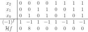
Let $H_n$ denote the $2^n\times 2^n$ Hadamard matrix defined by $(H_n)_{i,j} = (-1)^{b(i)\cdot b(j)}$ , for each $i,j$ such that $0\leq i,j\leq n-1$ . Inductively, these can be defined by

$H_1 = \left( \begin{array}{cc} 1 & 1\\ 1 & -1 \\ \end{array} \right), \ \ \ \ \ \ H_n = \left( \begin{array}{cc} H_{n-1} & H_{n-1}\\ H_{n-1} & -H_{n-1} \\ \end{array} \right), \ \ \ \ \ n>1.$
The Walsh-Hadamard transform of $f$ is defined to be the vector in ${\mathbb{R}}^{2^n}$ whose $k$ th component is

$({\mathcal{H}} f)(k) = \sum_{i \in \{0,1,\ldots,2^n-1\}}(-1)^{b(i) \cdot b(k) + f(b(i))} = (H_n (-1)^f)_k,$

where we define $(-1)^f$ as the column vector where the $i$ th component is

$(-1)^f_i = (-1)^{f(b(i))},$

for $i = 0,\ldots,2^n-1$ .

Example
A Boolean function of three variables cannot be bent. Let $f$ be defined by:

$\begin{array}{c|cccccccc} x_2 & 0 & 0 & 0 & 0 & 1 & 1 & 1 & 1 \\ x_1 & 0 & 0 & 1 & 1 & 0 & 0 & 1 & 1 \\ x_0 & 0 & 1 & 0 & 1 & 0 & 1 & 0 & 1 \\ \hline (-1)^f & 1 & -1 & 1 & -1 & 1 & -1 & 1 & -1 \\ {\mathcal{H}}f & 0 & 8 & 0 & 0 & 0 & 0 & 0 & 0 \\ \end{array}$
This is simply the function $f(x_0,x_1,x_2)=x_0$ . It is even because

$\Omega_f = \{ (0,0,1), (0,1,1), (1,0,1), (1,1,1) \},\ \mbox{ so } \ \omega = 4.$

Here is some Sage code verifying this:

sage: from sage.crypto.boolean_function import *
sage: f = BooleanFunction([0,1,0,1,0,1,0,1])
sage: f.algebraic_normal_form()
x0
sage: f.walsh_hadamard_transform()
(0, -8, 0, 0, 0, 0, 0, 0)

(The Sage method walsh_hadamard_transform is off by a sign from the definition we gave.) We will return to this example later.

Let $X=(V,E)$ be the Cayley graph of $f$ :

$V = GF(2)^n,\ \ \ \ E = \{(v,w)\in V\times V\ |\ f(v+w)=1\}.$
We shall assume throughout and without further mention that $f(0)\not=1,$ so $X$ has no loops. In this case, $X$ is an $\omega$ -regular graph having $r$ connected components, where

$r = |GF(2)^n/{\rm Span}(\Omega_f)|.$

For each vertex $v\in V$ , the set of neighbors $N(v)$ of $v$ is given by

$N(v)=v+\Omega_f,$

where $v$ is regarded as a vector and the addition is induced by the usual vector addition in $GF(2)^n$ . Let $A = (A_{ij})$ be the $2^n\times 2^n$ adjacency matrix of $X$ , so

$A_{ij} = f(b(i)+b(j)), \ \ \ \ \ 0\leq i,j\leq 2^n-1.$

Example:
Returning to the previous example, we construct its Cayley graph.

First, attach afsr.sage from [C] in your Sage session.

     sage: flist = [0,1,0,1,0,1,0,1]
     sage: V = GF(2)ˆ3
     sage: Vlist = V.list()
     sage: f = lambda x: GF(2)(flist[Vlist.index(x)])
     sage: X = boolean_cayley_graph(f, 3)
     sage: X.adjacency_matrix()
     [0 1 0 1 0 1 0 1]
     [1 0 1 0 1 0 1 0]
     [0 1 0 1 0 1 0 1]
     [1 0 1 0 1 0 1 0]
     [0 1 0 1 0 1 0 1]
     [1 0 1 0 1 0 1 0]
     [0 1 0 1 0 1 0 1]
     [1 0 1 0 1 0 1 0]
     sage: X.spectrum()
     [4, 0, 0, 0, 0, 0, 0, -4]
     sage: X.show(layout="circular")

In her thesis, Bernasconi found a relationship between the spectrum of the Cayley graph $X$ ,

${\rm Spectrum}(X) = \{\lambda_k\ |\ 0\leq k\leq 2^n-1\},$

(the eigenvalues $\lambda_k$ of the adjacency matrix $A$ ) to the Walsh-Hadamard transform $\mathcal H f = H_n (-1)^f$ . Note that $f$ and $(-1)^f$ are related by the equation $f=\frac 1 2 (e - (-1)^f),$ where $e=(1,1,...,1)$ . She discovered the relationship

$\lambda_k = \frac 1 2 (H_n e - \mathcal H f)_k$

between the spectrum of the Cayley graph $X$ of a Boolean function and the values of the Walsh-Hadamard transform of the function. Therefore, the spectrum of $X$ , is explicitly computable as an expression in terms of $f$ .

References:

[BC] A. Bernasconi and B. Codenotti, Spectral analysis of Boolean functions as a graph eigenvalue problem, IEEE Trans. Computers 48(1999)345-351.

[CJMP] Charles Celerier, David Joyner, Caroline Melles, David Phillips, On the Hadamard transform of monotone Boolean functions, Tbilisi Mathematical Journal, Volume 5, Issue 2 (2012), 19-35.

[S] P. Stanica, Graph eigenvalues and Walsh spectrum of Boolean functions, Integers 7(2007)\# A32, 12 pages.

Here’s an excellent video of Pante Stanica on interesting applications of Boolean functions to cryptography (30 minutes):

The mathematics of Midway

Posted on 2012/09/05 by wdjoyner

The battle of Midway was a historic turning point for the US during World War II. Joe Rochefort was the officer in charge of Station Hypo, a group of hand-picked Navy cryptographers tasked with breaking the Japanese Navy cipher. The machine the Japanese used was the JN-25. Unlike the British Bletchley Park cryptographers trying to break the Enigma traffic, he cryptographers did not have a version of the JN-25 machine. The fascinating story of Rochefort is explained brilliantly in the 2011 book “Joe Rochefort’s War” by Elliot Carlson.
Recently, Chris Christensen of Northern Kentucky University, one of the top historical experts on the US Navy cryptographers during WWII, have two lectures on the mathematics behind breaking the JN-25 ciphers.

45 minutes:

30 minutes:

Some remarks on monotone Boolean functions

Posted on 2012/09/01 by wdjoyner

This post summarizes some joint research with Charles Celerier, Caroline Melles, and David Phillips.

Let $f:GF(2)^n \to GF(2)$ be a Boolean function. (We identify $GF(2)$ with either the real numbers $\{0,1\}$ or the binary field ${\mathbb{Z}}/2{\mathbb{Z}}$ . Hopefully, the context makes it clear which one is used.)

Define a partial order $\leq$ on $GF(2)^n$ as follows: for each $v,w\in GF(2)^n$ , we say $v\leq w$ whenever we have $v_1 \leq w_1$ , $v_2 \leq w_2$ , …, $v_n \leq w_n$ . A Boolean function is called monotone (increasing) if whenever we have $v\leq w$ then we also have $f(v) \leq f(w)$ .

Note that if $f$ and $g$ are monotone then (a) $f+g+fg$ is also monotone, and (b) $\overline{\Omega_f}\cap \overline{\Omega_g}=\overline{\Omega_{fg}}$ . (Overline means bit-wise complement.)

Definition:
Let $f:GF(2)^n \to GF(2)$ be any monotone function. We say that $\Gamma\subset GF(2)^n$ is the least support of $f$ if $\Gamma$ consists of all vectors in $\Omega_f$ which are smallest in the partial ordering $\leq$ on $GF(2)^n$ . We say a subset $S$ of $GF(2)^n$ is admissible if for all $x,y\in S$ , ${\rm supp}(x)\not\subset {\rm supp}(y)$ and ${\rm supp}(y)\not\subset {\rm supp}(x)$

Monotone functions on $GF(2)^n$ are in a natural one-to-one correspondence with the collection of admissible sets.

Example:
Here is an example of a monotone function whose least support vectors are given by
$\Gamma =\{ (1,0,0,0), (0,1,1,0), (0,1,0,1), (0,0,1,1) \} \subset GF(2)^n,$
illustrated in the figure below.

The algebraic normal form is $x_0x_1x_2 + x_0x_1x_3 + x_0x_2x_3 + x_1x_2 + x_1x_3 + x_2x_3 + x_0$ .

The following result is due to Charles Celerier.

Theorem:
Let $f$ be a monotone function whose least support vectors are given by $\Gamma \subset GF(2)^n$ . Then
$f(x) = 1+\prod_{v\in\Gamma} (x^v+1).$

The following example is due to Caroline Melles.

Example:
Let $f$ be the monotone function whose least support is
$\Gamma = \{ (1,1,1,1,0,0),(1,1,0,0,1,1),(0,0,1,1,1,1)\}.$
Using the Theorem above, we obtain the compact algebraic form
$f(x_0,x_1,x_2,x_3,x_4,x_5) = x_0x_1x_2x_3 + x_0x_1x_4x_5 + x_2x_3x_4x_5 .$
This function is monotone yet has no vanishing Walsh-Hadamard transform values. To see this, we attach the file afsr.sage available from Celerier (https://github.com/celerier/oslo/), then run the following commands.

sage: V = GF(2)^(6)
sage: L = [V([1,1,0,0,1,1]),V([0,0,1,1,1,1]), V([1,1,1,1,0,0])]
sage: f = monotone_from_support(L)
sage: is_monotone(f)
True

These commands simply construct a Boolean function $f$ whose least support are the vectors in L. Next, we compute the Walsh-Hadamard transform of this using both the method built into Sage’s sage.crypto module, and the function in afsr.sage.

sage: f.walsh_hadamard_transform()
(-44, -12, -12, 12, -12, 4, 4, -4, -12, 4, 4, -4, 12, -4, -4, 4, -12, 4, 4, -4, 4, 4, 4, -4, 4, 4, 4, -4, -4, 
 -4, -4, 4, -12, 4, 4, -4, 4, 4, 4, -4, 4, 4, 4, -4, -4, -4, -4, 4, 12, -4, -4, 4, -4, -4, -4, 4, -4, -4, -4, 4, 4, 4, 4, -4)
sage: f.algebraic_normal_form()
x0*x1*x2*x3 + x0*x1*x4*x5 + x2*x3*x4*x5
sage: x0,x1,x2,x3,x4,x5 = var("x0,x1,x2,x3,x4,x5")
sage: g = x0*x1*x2*x3 + x0*x1*x4*x5 + x2*x3*x4*x5
sage: Omega = [v for v in V if g(x0=v[0], x1=v[1], x2=v[2], x3=v[3],
     x4=v[4], x5=v[5])0]
sage: len(Omega)
10
sage: g = lambda x: x[0]*x[1]*x[2]*x[3] + x[0]*x[1]*x[4]*x[5] + x[2]*x[3]*x[4]*x[5]
sage: [walsh_transform(g,a) for a in V]
[44, 12, 12, -12, 12, -4, -4, 4, 12, -4, -4, 4, -12, 4, 4, -4, 12, -4, -4, 4, -4, -4, -4, 4, -4, -4, -4, 4, 4, 
 4, 4, -4, 12, -4, -4, 4, -4, -4, -4, 4, -4, -4, -4, 4, 4, 4, 4, -4, -12, 4, 4, -4, 4, 4, 4, -4, 4, 4, 4, -4, -4, -4, -4, 4]

(Note: the Walsh transform method in the BooleanFunction class in Sage differs by a sign from the standard definition.) This verifies that there are no values of the Walsh-Hadamard transform which are $0$ .

More details can be found in the paper listed here. I end with two questions (which I think should be answered “no”).

Question: Are there any monotone functions $f$ of $n$ variables having no free variables of degree $\leq n/2$ ?

Question: Are there any monotone functions $f$ of most than two variables which are bent?

Review of R. Beezer’s “A first course in linear algebra”

Posted on 2012/08/01 by wdjoyner

The book this review will look at, A first course in linear algebra by Robert Beezer, is remarkable for several reasons. First, it is free and you can download it from its website. Second, if you have a somewhat different approach to teaching linear algebra and prefer a slightly modified version, you are in luck: Beezer’s book is open source, so you can download the LaTeX source, change it to suit your needs (delete some material and/or add some of your own), and then redistribute your revised version according to the stipulations of the GNU Free Documentation License. If are unsure how to do this, or have any book-related question, you’re in luck again – there is a googlegroups email list to help you out. Finally, it is huge. The version I will review (version 2.0) is not the most recent (at the time of this writing, version 3.0 is almost out) but still the book was about 750 pages (the most recent version is over 1000 pages!). There is plenty of material to fit almost any syllabus.

Cover of Beezer’s linear algebra book

Speaking of material, what does this book actually cover? The chapters are:

[SLE]
Systems of linear equations
[V]
Vectors
[M]
Matrices
[VS]
Vector spaces
[D]
Determinants
[E]
Eigenvalues
[LT]
Linear transformations
[R]
Representations

There are also several appendices (for example, one on Sage a free and open source mathematics software program with very strong linear algebra computational capabilities [S]).

Note the unusual labeling of the chapters – no numbering is used for the chapters, instead capital Roman letters are used (an acronym, E for Eigenvalues, for example). The same indexing method is used for the definitions, examples and theorems as well. How do you refer to a result with this method of labeling? The way cross-referencing works in this book is that each reference is followed by the page number that the reference can be found. For example the theorem that says the adjoint of a matrix respects matrix addition would be referred to as “Theorem AMA [175]” since it can be found on page 175 and is written there as

Theorem AMA (Adjoint and Matrix Addition):
Suppose $A$ and $B$ are matrices of the same size. Then $(A+B)^T = A^T + B^T$ .

One advantage to this method of indexing is that if, for example, replace the chapter on Vectors with your own chapter then recompile the LaTeX, the theorem on adjoint and matrix addition is still “Theorem AMA,” even though its page number has probably changed. Although this indexing method with the page numbers does make the various results pretty easy to find, all the labeled results are also conveniently listed in the index. Moreover, in the the electronic versions (PDF, XML, jsMath) of the book, all of this cross-referencing is available as hyperlinks.

Each chapter of course is composed of many sections. Each section not only has plentiful detailed examples and its own list of “reading questions” to see if you have understood the material, but also a list of exercises with solutions. More precisely, some exercises are marked as computational (e.g., solve the following system of linear equations), some as theoretical (e.g., prove that if a vector v is in the kernel of a matrix then any scalar times v is also in the kernel), and some as “mixed” (often of the form: find an example of a matrix with property X). As far as I could see, every computational exercise was accompanied by a more-or-less complete solution. However, the other types of problems usually (not always) either had no solution provided or only a sketch of one. A rough count would be about 500 exercises and 350 of them have solutions.

The book is very well-written and at a level similar to Anton’s popular book \cite{A}. What topics are actually covered by this book? There is a detailed table of contents of (a) the chapters, sections and subsections, (b) the definitions, (c) the theorems, (d) the examples, and (e) a 30 page index.

The first chapter on systems of linear equations discusses solving systems of linear equations, as well as classifying them (consistent, homogeneous, and so on), row reduction, and the matrix form of a system of linear equations. This chapter, in my opinion, approaches things in the right way by stressing the importance of the method of row reduction/Gauss elimination. Very detailed proofs are also presented. For most students, the more details the better, so this is also a strong plus.

The second chapter on vectors starts with the basics on vector operations. This is followed by four sections on linear spans and linear independence. This is a challenging topic for students but the book does a very though job. The final section discusses orthogonality, inner products and the Gram-Schmidt procedure.

The chapter on matrices comprises six sections. After several sections explaining the usual details on matrix operations (such as transposes and adjoints) and matrix arithmetic (such as addition and multiplication), the discussion turns to matrix inverses. Two sections are spent with this topic. The last two sections deal with row and column spaces and their basic properties.

The chapter on vector spaces begins with two sections on the basic definitions and properties of vector spaces and subspaces. The next two sections are on linear independence (again), spanning sets (again), and vector space bases. With the difficulty that linear independence and spanning sets present to many students, this reappearance of these topics provides excellent reinforcement. The last sections of the chapter are on the dimension properties of the row-span and column span of a matrix. For example, what Gilbert Strang calls the Fundamental Theorem of Linear Algebra, the so-called “rank plus nullity theorem,” is in one of these sections (see Theorem RPNC in section RNM on page 323).

After a relatively short 24-page chapter on the determinant and its properties, the book continues with the Eigenvalues chapter. This chapter discusses eigenvalues, eigenvectors, diagonalization, and similarity. Topics such as the Jordan canonical form are discussed in a later chapter.

The chapter on linear transformations has separate sections on injective maps, surjective maps, and invertible maps, resp.. This chapter has a wealth of examples to help guide the student through these relatively abstract concepts.

The final chapter is also the most difficult for the student. This is the chapter titled Representations, concerning topics such as the matrix representation of a linear transformation and the properties of this representation. Other topics, such as the Cayley-Hamilton Theorem, the Jordan canonical form, and diagonalization of orthogonal matrices appear in this chapter as well. In version 2.0, some sections of this chapter were less complete than those in other chapters.

Finally, I would also like to mention that the author has done a considerable amount of work on the use of Sage in the classroom. For example, he has added to the Sage code and documentation and has written the following “quick reference sheets” summarizing the most useful linear algebra commands in Sage. For more information, see his website http://linear.ups.edu/sage-fcla.html.

An excellent book written by an experienced teacher. Highly recommended.

Bibliography:

[A] H. Anton, Elementary linear algebra, 8th edition, Wiley, 2000.

[B] Robert Beezer’s Linear Algebra website, http://linear.ups.edu/.

[S] W. Stein, Sage: Open Source Mathematical Software (Version 5.2), The Sage~Group, 2012, http://www.sagemath.org

Ahlfors and Beurling

Posted on 2012/07/28 by wdjoyner

This is an exposition on Ahlfors and Beurling, two mathematicians I admire. There is nothing original at all. Everything below is collected from Beckman’s excellent book [B], Wikipedia, and papers which I found on the internet using google searches.

The universe consists of Nine Worlds which are resting on an immense tree called Yggdrasil. Asgard is one of the Nine Worlds and is the country of the Norse Gods. Asgard is a land more fertile than any other, blessed also with a great abundance and its people excelled beyond all others in strength, beauty and talent. Odin is a major god and the ruler of Asgard. Odin has many great sons, among them, the brothers Baldur and Tyr. – Nortic legend

The tree Yggdrasil

Lars Ahlfors and Arne Beurling are among the greatest mathematicians in history. Eventually, they became became collaborators in research, and the best of friends.

Ahlfors

Baldur (or Baldr, Balder) is the god of innocence and piety. So bright and fair he is that light shines from his features. He is wise, eloquent, gentle, and righteous to such a degree that his judgments stand always unshaken. – Norse Legend

Finland was a part of Sweden from the 12th to 19th century and from 1809 to 1917 was part of the Russian Empire, although given some autonomy. The Parliament of Finland passed a Declaration of Independence from Russia in 1917, approved a month or so later by the Russian government. Finland fought World War II as essentially three separate conflicts:

the Winter War (1939-40), against the Soviet Union which forced Finland to cede 11% of its pre-war territory and 30% of its economic assets to the Soviet Union,
the Continuation War (1941-44), against the Soviet Union which forced Finland to pay $ 226,500,000 in reparations to the Soviet Union, while ultimately retaining its independence, and
the Lapland War (1944-45), against Nazi Germany.

Lars Ahlfors was born in Helsinki, Finland in 1907 during a time when Finland was under Russian rule. Sadly, his mother died in childbirth. His father was a Professor of Engineering at the Helsinki University of Technology. Ahlfors studied at University of Helsinki from 1924, graduating in 1928 having studied under Ernst Lindelöf and Rolf Nevanlinna. (Nevanlinna replaced Weyl in Zurich for the session 1928/29 while Weyl was on leave, and Ahlfors went to Zurich with him.) He completed his doctorate from the University of Helsinki in 1930. After he presented his doctoral thesis in 1930, he made a number of visits to Paris and other European centers from 1930-1932. He also taught (in Swedish) at Aaboe Academy in Turku from 1929 to 1932.

Ahlfors worked as an Associate Professor at the University of Helsinki from 1933 to 1936. In 1935-1938 Ahlfors visited Harvard University. From 1938-1943 he was a professor at the University of Helsinki.

As a Finn, he was required to serve in the military, for which he worked in a bomb shelter.

World War II presented many problems for Ahlfors and his wife and children. Due to travel restrictions and threats to his family, his wife and children left for Sweden early in the war, leaving Ahlfors behind. He left when he could and was professor at the Swiss Federal Institute of Technology at Zurich from 1945-1946 (he was only there for 1 year, though he was offered the post earlier). From 1946-1977, Ahlfors was professor at Harvard. He was the William Caspar Graustein Professor of Mathematics of Harvard from 1964-1977.

In 1936, the year the first Fields medals were awarded, he was one of the first two people to be given the Medal. He was an invited speaker at the ICM in 1962 and in 1978. He was selected for the Wihuri Sibelius Prize [W] in 1968, the Wolf Prize in Mathematics in 1981, and the AMS Steele Prize in 1982.

For a student of mathematics, a common introduction to Ahlfors was by reading his classic textbook on complex analysis which is still very highly regarded. It was Complex Analysis: an Introduction to the Theory of Analytic Functions of One Complex Variable.

Ahlfors’ first famous result was his proof of Denjoy’s conjecture, discussed next. If $f:{\mathbb{C}} \to {\mathbb{C}}$ is a function, the function $M(r, f) = \max_{0\leq \theta\leq 2\pi} |f(re^{i\theta} )|$ is called the maximum modulus of $f$ . The order of $f$ is

$\rho= \limsup_{r\to\infty} \frac{\log\log M(r,f)}{\log r}.$

For example, if $f(z) = e^{z^k}$ then we have $\rho=k$ . We say $f$ has an asymptotic value $\alpha$ if there is a curve $\Gamma$ connecting $0$ to $\infty$ such that $f (z) \to \alpha$ as $z \to \infty$ on $\Gamma$ . Denjoy (1907) asked the question “if $f$ has $k$ distinct finite asymptotic values, is the order of $f$ greater than or equal to $k/2$ ?” In his PhD thesis, Ahlfors proved the answer is yes.

Ahlfors also worked with Beurling on several papers, which shall be discussed below. Later in his career, Ahlfors worked on Kleinian groups, sometimes in collaboration with Lipman Bers.

A Kleinian group $G$ is a discrete subgroup of $PSL(2, {\mathbb{C}}).$ The group $PSL(2, {\mathbb{C}})$ of $2 \times 2$ complex matrices of determinant $1$ modulo its center may be represented as a group of conformal transformations of the Riemann sphere. The boundary of the closed ball is called the sphere at infinity, and is denoted $S_\infty$ . Consider $G$ as orientation preserving conformal maps of the open unit ball $S_\infty$ in ${\mathbb{R}}^3$ to itself. The orbit $Gp$ of a point $p$ will typically accumulate on the boundary of the closed ball. The set of accumulation points of $Gp$ in $S_\infty$ is called the limit set of $G$ . A Kleinian group is said to be of type $1$ if the limit set is the whole Riemann sphere, and of
type $2$ otherwise.

One of Ahlfors’ most well-known results is his “finiteness theorem,” which says that the ordinary set $\Omega$ of a (finitely generated) Kleinian group $G$ factored by the action of the group is an orbifold $\Omega/G$ of finite type. In other words, $\Omega/G$ has finitely many “marked” points and can be compactified by adding a finite number of points.

Ahlfors has remarked that perhaps of greater interest than the theorems that he has been able to prove were the ones he was not able to prove. For example, there is the assertion that the limit set of a finitely generated Kleinian group has two-dimensional Lebesgue measure zero. This has become known as the Ahlfors measure zero conjecture. It is still unsolved.

Beurling

Tyr is the god of war and he does nothing whatever for the promotion of concord. Tyr is bold and courageous – men call upon him in battle, and he gives them courage and heroism.

The eastern half of Sweden, present-day Finland, was lost to Russia in 1809. The last war in which Sweden was directly involved was in 1814, when Sweden by military means forced Norway into a personal union. Since then, Sweden has been at peace, practicing “non-participation in military alliances during peacetime and neutrality during wartime.”

During the German invasion of the Soviet Union, Sweden allowed the Wehrmacht to use Swedish railways to transport (June-July 1941) the German 163rd Infantry Division along with howitzers, tanks and anti-aircraft weapons and associated ammunition, from Norway to Finland. German soldiers traveling on leave between Norway and Germany were allowed passage through Sweden. Iron ore was sold to Germany throughout the war. And for the Allies, Sweden shared military intelligence and helped to train soldiers made up of refugees from Denmark and Norway. It also allowed the Allies to use Swedish airbases between 1944 and 1945.

Arne Carl-August Beurling (February 3, 1905 – November 20, 1986) was a Swedish mathematician and professor of mathematics at Uppsala University (1937-1954) and later at the Institute for Advanced Study in Princeton, New Jersey.

He was awarded the Swedish Academy of Sciences Prize 1937 and 1946, the Celsius Gold Medal 1961, and the University of Yeshiva Science Award 1963. In his honor a “Beurling Year” was held at the Mittag-Leffler Institute (Beurling was offered the directorship of the MLI but turned it down…) in Stockholm 1976/77.

Family: Father – Konrad Beurling; Mother – Elsa Raab Beurling (who divorced Konrad in 1908 and went back to using Baroness Elsa Raab); Great grandfather (on father’s side) – Pehl Beurling, whose father was a famous clock-maker. According to Beckman [B], Konrad had 14 children in wedlock, and “an unknown number” out of wedlock. (I don’t know if “unknown” means Konrad didn’t know or Beckman didn’t know:-)

Arne graduated high school in 1924 and went to the university in Uppsala. He got his undergaduate degree in 1926, masters in 1928.

In 1925 the Swedish General Staff contacted a commercial company to design a machine that would be superior to the German Enigma. Hagelin developed a prototype for evaluation called the B21. The B21 was approved for the Swedish General Staff and Hagelin also sold the machine to several other countries.

While working on his PhD, Beurling did his military service, excelling in a course in military cryptanalysis. In fact, this is a considerable understatement. Towards the end of the course, the instructor, a Naval officer named Anderberg, brought in a commercial crypto-machine, the Hagelin B21. The graduate student Beurling modestly asked if he could examine the machine over the weekend. The instructor okayed this simple request. The following Monday, Beurling told Anderberg that the machine had a weakness. Anderberg denied this claim and challenged him with a long crib. Beurling promply decrypted it, stunning Anderberg.

Some of Beurling’s other cryptographic feats:

Beurling broke the Geheimschreiber without having a copy of the
machine (see pp. 43-86 of Beckman [B]). (As the Geheimschreiber encrypted very high-level Nazi traffic, the military significance of this cannot be underestimated.)
Beurling broke several encrypted telegrams in Czech,
a language he did not know (see pp. 109-113 in Beckman [B]).

In mid-June 1941 Sweden told Great Britian of Germany’s plan to attack the Soviet Union, the attack to commence in late June 1941 (“Operation Barbarossa” – see pp. 120-121 in Beckman [B]). A spy then communicated this information to the Soviet Union (see Ulfving and Weierud [UF], page 22). At the time, the Soviets did not believe the information, thinking the British were only trying to trick them into attacking the Germans.

Beurling started teaching in the mathematics department of Uppsala University in 1932. His PhD was defended in 1933, though most of it was written much earlier. (He went on a long hunting trip with his father to Panama. Also, he did his military service at this time.) Beurling’s thesis contained a proof of the Denjoy conjecture, whose proof was found independently and published in his PhD by Ahlfors a few years earlier. Except for visiting positions, he stayed at Uppsala until he left to go to the Institute for Advanced Study in the 1950s.

A photo of Beurling taken by Annette-Marie Yxkull.

Consider a plane region $D$ and let $E$ be a subset of the boundary of $D$ . Consider a harmonic function in $D$ , denoted by $\omega (z,E,D)$ and known as the harmonic measure at $z$ of $E$ with respect to $D$ . It is defined by having boundary values $1$ on $E$ and $0$ on the rest of the
boundary. If it is known that $|\log f(z)|\leq \omega$ on the whole boundary, then, by the maximum principle, $|\log f(z_0)|\leq \omega(z_0,E, D)$ , for every interior point $z_0$ .

A difficult and important result is Beurling’s estimate for the harmonic measure expressed through the inequality

$\omega \leq \exp(-\lambda^2+1),$
where $\lambda =\lambda (z_0, E, D)$ is the extremal distance between $z_0$ and the boundary set $E$ . If $E$ is conformally equivalent to an arc on the unit circle there is also an opposite inequality

$\omega \geq \exp(-\lambda^2).$
These inequalities were strong enough for a proof of the Denjoy conjecture (independent of that of Ahlfors) concerning the number of asymptotic values of an entire function of finite order.

This may be Beurling’s most famous theorem: Let $H^2$ be the Hilbert space of holomorphic functions in the unit disk which belong to $L^2$ on $|z|= 1$ . Let $E$ be a closed subspace, invariant under multiplication by $z$ . Then there exists an inner function $\phi(z)$ , i.e. $|\phi(z)|<1$ , $|\phi(e^{i\theta})|=1$ a.e., such that $f\in E$ if and only if $f=\phi\cdot f_0$ , with $f_0\in H^2$.

Beurling’s first paper in harmonic analysis is an extension of the prime number theorem to generalized primes. Let $P: 1<p_1<p_2< \dots$ be the given sequence of "primes" and let

${\mathbb{Z}}_P = \{ p_1^{a_1}\dots p_k^{a_k}\ |\ a_i\in {\mathbb{Z}}\}$
be the "integers". Let $\pi_P (x)$ and $N_P(x)$ be the corresponding counting functions. Then $|N_P(x)-ax| 0$ , implies the prime-number theorem $\pi_P(x)\sim x/\log x$ if $\gamma >3/2$ but in a sense not if $\gamma <3/2$ .

If $P$ satisfies $\pi_P(x)\sim x/\log x$ then we call $P$ a Beurling prime number system. A question raised by Beurling remains open: what functions $E(x)$ are such that $|N_P(x)-x|0$ , then Olofsson [O] conjectures that

$\limsup_{x\to\infty} \frac{N_P(x)-x}{\ln x} >0,$
provided $P$ is different from the rational primes. Olofsson conjectures that Beurling’s question is addressed by any function $E(x)$ satisfying $E(x)=o(\ln x)$ .

This is just a small sampling of Beurling’s brilliant work.

Ahlfors and Beurling

Ahlfors once wrote “Arne Beurling was the best friend I ever had.” Ahlfors enjoyed the quiet life of a writer and mathematician, whereas Beurling loved the outdoors, sailing, hunting. They first met in 1934 at the Scandanavian Congress of Mathematicians held in Stockholm. They were both still single, although Ahlfors would marry the following year. Beurling had just gotten his PhD the previous year. After the 1934 Congress, while Ahlfors was still at Mittag-Leffler, he would often take the train up to Uppsala to visit Beurling. Much later, when Ahlfors was at Harvard, Beurling’s girlfriend Annette-Marie Yxhull wrote Ahlfors a latter, explaining how unhappy Beurling was at Uppsala (see Beckman [B]). Ahlfors acted quickly, obtaining a visiting position for his friend at Harvard. Later, Beurling was given a permanent position at the Institute for Advanced Study, no doubt with Ahlfors’ strong recommendation.

A photo of Ahlfors taken by A. Beurling.

Beurlings work with Ahlfors was in the field of quasiconformal mappings. Let $f:D \to D'$ be an orientation-preserving homeomorphism between open sets in the plane. If $f$ is continuously differentiable, then it is $K$ -quasiconformal if the derivative of at every point maps circles to ellipses with eccentricity bounded by $K$ . We say $f$ is quasiconformal if $f$ is $K$ -quasiconformal for some finite $K$ .

A quasiconformal map.

According to Ahlfors, in their joint paper [AB], the decisive idea was entirely due to Beurling. It deals with the boundary values of quasiconformal mappings. If $h(x)$ increases for $-\infty <x1$ ,

$1/\rho \leq \frac{h(x+t)-h(x)}{h(x)-h(x-t)} \leq \rho,$
for all $x$ and $t$ .

Bibliography

[AB] L. V. Ahlfors and A. Beurling, The boundary correspondence under
quasi-conformal mappings, Acta Math., 96 (1956), 125-142.

[B] B. Beckman, Codebreakers, AMS, 2002.

[O] R. Olofsson, Properties of the Beurling generalized primes, preprint, 2008.

[UF] The Geheimschreiber Secret, by Lars Ulfving, Frode Weierud, in Coding Theory and Cryptography: From Enigma and Geheimschreiber to Quantum Theory, Springer-Verlag, 2000.
paper in pdf or link at Frode’s cryptocellar

[W] Wihuri Sibelius Prize

The man who found God’s number

Posted on 2012/07/06 by wdjoyner

(added Sep. 2014: An updated version of this article will appear in the College Math Journal.)

We have an appetite for information, and especially for pattern, information that falls into meaningful arrays from which we can make rich inferences. Information can be costly to obtain and analyze, but because it offers an invaluable basis for action, nature evolves senses and minds to gather and process information appropriate to particular modes of life. Like other species, humans can assimilate information through the rapid processing that specialized pattern recognition allows, but unlike other species we also seek, shape, and share information in an open-ended way. Since pattern makes data swiftly intelligible, we actively pursue patterns…

Brian Boyd
(On the Origin of Stories, [B])

Introduction

The Rubik’s cube was a world-wide obsession in the early 1980, when Tomas Rokicki, a high school junior in Texas, got his first one. Around the same time, Tom began losing his sense of hearing.

During the 1980s there were Rubik’s cube solving contests (some even televised) but no one knew the smallest number of moves needed to solve the cube. This mysterious quantity, “God’s number,” was the number of moves needed to solve the cube in its most scrambled state. Although David Singmaster, cubologist extraordinaire, guessed it might be in the low 20s, no one had a serious conjecture as to what God’s number would actually be. The cube solving contest winners relied on knowing various solving strategies and very fast finger movement.

During that era, hearing aids were very primitive and no one knew how to restore hearing to those who were totally deaf. In the 1970s-1980s, hearing aids were so-called “in the ear” transistor devices. By the time Tom got his first one in the 1980s, they were small earbuds which fit inside the ear, but not reaching into the ear canal [T]. Unfortunately, the device was useless unless you had at least some hearing ability.

We do know, thanks to Tom Rokicki’s recent work, the value of God’s number (explained below). This was a very difficult problem to solve. Also, we do know, due to decades of work by many researchers, how to restore hearing to the totally deaf [W]. Thanks to two double cochlear implant surgeries, that Tom’s hearing is almost fully restored. Digitizing human hearing is a very difficult problem to solve.

The Rubik’s cube

The Rubik’s cube, or simply the cube for short, was unleashed on the world in the
mid 1970’s. It became a sensation world-wide but is still remains a popular mechanical puzzle for people of all ages. For the sake of orientation, here is a short description. Image a cube sitting on a table. This cube has six faces: up, down, left, right, front and back. Color each of the six faces with a different color. Now cut up the cube into 27 subcubes of equal size using slices parallel to the faces. In the mid 1970s, Erno Rubik, a Hungarian professor of architecture and design at a university in Budapest, did just this but also figured out an ingenious internal mechanism for connecting the 26 external subcubes in a way that allows them to be rotated around a center. This mechanism allows each face to be rotated by $90^o$ or $180^o$ or $270^o$ , clockwise or counterclockwise. The effect of this is that the centers of the faces do not change. If you imagine the front face of the cube as always facing you and that you are holding the cube with your right hand on the right face, the the total number $N$ of different positions that the cube could be scrambled is

$N = 8!\cdot 12!\cdot 2^{10}3^7=43252003274489856000 \cong 4.3\times 10^{19},$
or about 43 billion billion positions (see [J]). In the sense of Brian Boyd’s quotation, the Rubik’s cube is full of “patterns.”

Imagine having to search through this. How does it compare with finding a needle in a haystack? A straw of hay is about 1 gram. For a 200 pound haystack, that works out to about $100000=10^4$ straws in a haystack. In other words, finding a needle in a haystack is $10^{14}$ (“ten thousand billion”) times easier. How does it compare to the gross domestic product of the United States economy? This number $N$ is over one million times the size of the United States GDP. How does it compare to the distance to the moon in the sky? If you stacked sheets of paper on top of each other until their thickness grew to the moon, the number of sheets you uses would be over a million times smaller than this number $N$ . How does it compare to searching the largest publically known database that arose in commerce or government? The largest such database is at the World Data Centre for Climate [F], weighing in at about $6$ petabytes, or $6\times 10^{15}$ . Imagine having to search through this. The “Rubik’s cube database” is over $1000$ times larger. This number of cube positions is a very big number. This is what Tom is trying to search through.

I do not recall who gave me the cube, but I do remember quite clearly trying to solve it, and being surprised at how difficult it was. For months I tried to solve it, on and off, and just could not restore it; I could get two layers, but the last layer was just too difficult. Finally, I started keeping a notebook on the cube, and looked for some sequences (algorithms, I now know they are called) that would affect only a small portion of the cube, leaving the rest alone. At one point I had all the algorithms I needed except the one that permuted three corners. With a bit more work I finally figured out those pesky corners, and had a full solution. It took me about six months from originally getting the cube until this point! I did top corners first, then bottom corners, then top and bottom edges, and finally middle edges.

– Tom Rokicki

Since the late 1970’s, mathematicians and computer scientists have been wondering how many moves do you need to make to solve the Rubik’s cube, in the worst case scenario. There are two ways to measure the number of moves you make while manipulating the cube. One is called the quarter-turn metric. In this measurement, each quarter turn of any face of the cube, whether clockwise or counterclockwise, is called one move. The other is the face-turn metric. In this measurement, each turn of any face of the cube, whether by $90^o$ or $180^o$ or $270^o$ in either direction, is called one move. The use of the word “metric” is designed to suggest distance. How far from the solved position of the cube can you get? Starting from the solved position, how many moves would you have to make to scramble the cube into a position which is further from that solved position than any other? The answer depends on which metric you use. The exact answer is known as God’s number in the face-turn metric (resp., in the quarter-turn metric, if you prefer that measurement).

The determination of God’s number was the Mount Everest of mathematical questions
connected with the Rubik’s cube. With over $4.3\times 10^{19}$ possible positions, one might think that God’s number could be very large.

Hearing loss

The human ear is a complicated organ. In rough terms, here is how the hair cells in the inner ear contribute to hearing. Sound is basically a vibration of the molecules of the air created by small differences in air pressure. Different sound frequencies create different pressure differences. Deep inside the ear, in an area called the cochlea, is a surface called the basilar membrane of the inner ear. In very rough terms, you can think of this surface as like your skin with hair on it. When it experiences a sound, the hair on it will vibrate. Remarkably, different frequencies will cause hair in different locations on this surface to vibrate. It is as though a high-pitched frequency would vibrate the hair on your legs and not your arms, but a low-pitched frequency would vibrate the hair on your arms and not your legs. This “frequency-to-place” mapping is the way the ear sorts out different frequencies, enabling our brain to process that sound. In a normal ear, high-frequency sounds are registered by the hair cells located at the shallower end of the cochlea, but low frequency sounds are registered by the hair cells further inside. When these hair cells vibrate, they create a tiny electrical impulse which the nerve cells in the basilar membrane pass to the brain. The brain interprets this activity to determine which sound frequency is being heard.

If you lack hair cells, then this process completely breaks down and you cannot distinguish frequencies. The most beautiful music is merely noise.

Tom’s hearing

As Michael Chorost explains in his book Rebuilt [Ch], some teenagers in the 1980s developed hearing problems due to the fact that, in the United States, there was a Rubella outbreak in the 1960s. One of the consequences of this virus
was that some pregnant women exposed to Rubella gave birth to babies who were more likely to gradually lose cochlear hair cells starting in the 1980s during their teenage years. However, other illnesses can cause hearing loss and the cause of Tom’s hearing problems is not known.

Tom graduated from Wolfe City High School in 1981, got a bachelors degree in electrical engineering from Texas A+M University in 1985, and a Ph.D. at Stanford University in Computer Science in 1993. While this was going on, Tom was becoming deaf. Here is how he describes it:

I am post-lingually progressively deafened. I started losing my hearing in high school (no cause is known), and in college it became a huge problem. A very good friend’s parents noticed how deaf I was and sprung for hearing aids for me (I was working my way through school at the time; no way I could afford them) and they helped a lot but school was still a challenge. Once I started working full-time I could afford more and better hearing aids, but as the aids got better my hearing got worse, until I reached a point that hearing aids weren’t really helping much at all.

Recent progress on God’s number

As long ago as the early 1980’s it was known that every position the cube could be solved in $52$ moves or less [C20]. Here is a table of progress since then.

	Lower	Upper
Date	bound	bound	Notes and Links
July, 1981	18	52	Morwen Thistlethwaite
Dec., 1990	18	42	Hans Kloosterman
May, 1992	18	39	Michael Reid
May, 1992	18	37	Dik Winter (just one day later!)
Jan., 1995	18	29	Reid (analyzing
			Kociemba’s two-phase algorithm).
Jan., 1995	20	29	Reid: the “superflip” position
			(This is the position of the Rubik’s cube where the centers and corners are correct, and all edges are correctly placed but “flipped.”) requires 20 moves.
April, 2006	20	27	Silviu Radu
May, 2007	20	26	Dan Kunkle and Gene Cooperman
March, 2008	20	25	Tomas Rokicki
Aug., 2008	20	22	Rokicki and John Welborn
July, 2010	20	20	Rokicki, Herbert Kociemba, Morley Davidson,
			and John Dethridge determine God’s number!

For years, Tom Rokicki has been working on lowering the upper bound for the face turn metric of the Rubik’s cube. His main work (finished in March 2008) is described in [TR], using a mathematical field known as group theory and prodigious programming skills. In Tom’s own words:

In December of 2003 I decided to solve the “edges-with-centers” space (the entire space of Rubik’s cube, ignoring all the corners). I wrote all of the code in C++ using a new set of classes for representing positions, sequences, and symmetry. The program itself required only 1.3GB of RAM, and I posted the results to the Yahoo newsgroup speedsolving in January 2004. This was the largest such complete implicit graph search performed to date at that time, I believe, with 980 billion states (before symmetry and antisymmetry reductions).

In November of 2005, I got an email from Silviu Radu that he had used the “edges-with-centers” results I had posted to lower the upper bound on God’s number in the quarter turn metric to 38. This email started a collaboration that, in the end, led to all the rest of the work. My debt to Silviu is profound.

Many others were also working on this problem, but Rokicki’s progress in early 2008 was so significant that Rubik’s cube aficiadados started to think Rokicki was about to make a first ascent on their own Mount Everest. In fact, it was soon afterwards that Sony’s John Welborn contacted Tom out of the blue and offered CPU time on the “farm” of computers which Sony Imageworks uses to render animated movies, such as “Spiderman 3.” As a result of this generous offer by Sony, Tom was able to extend the same method used in the $25$ -move upper bound to show, in the face turn metric, every position can be solved in $\leq 22$ moves.

Then Google called. They donated time on a supercomputer to rule out the cases $N=21,22$ . This meant God’s numbr was $\leq 20$ . On the other hand, the “superflip” position is known to take $20$ face moves exactly (Michael Reid established this in 1995), so $20$ is best possible. In other words, God’s number in the face turn algorithm is $20$ . What Tom did was great but, with a little help from some friends, an amazing milestone was achieved.

Cochlear implants

What a cochlear implant tries to do is generate tiny electrical impulses in the nerve cells of the basilar membrane by attaching small electrical wires to different locations where hair cells should be. Even though the cochlear implant is very small, it cannot match mother nature. In a normal human ear, there are about $20000$ hair cells. There is no way to surgically implant $20000$ electrical nodes in the small area of the human skull where the inner ear is located. However, even 25 electrodes, which is the current state of the art, can transform a deaf person’s life from noise (or silence) to meaningful sound. The implanted electrodes get “mapped” or “programmed” to nerve cells of the basilar membrane by an audiologist working closely with the patient. For some patients, the process of installing and mapping a functioning “bionic ear” goes fairly smoothly. For others, it can be a very frustrating experience.

How does the cochlear implant distinguish the frequencies which are then passed to the implanted electrodes? Sound waves can be “decomposed” into more basics sounds called fundamental harmonics. As a rough analogy, think of the sound from a piano chord, which can be decomposed into the sounds of its individual keys. Each of the individual piano keys makes a more fundamental, pure sound. Play them simultaneously, as you do when playing a piano chord, and you get a more complicated sound. Now, try to reverse this process. Listen to the sound of a complicated chord. How do you tell what the individual notes are? Assuming you are not a musician who knows the chords by heart, this question of decomposing a chord into individual key notes is a complicated one. Abstractly, the process of decomposing sound into fundamental harmonics uses the mathematics of Fourier analysis, a method physicists and mathematicians have known since the 1800s. However, mathematics and engineering are not the same. Implementing these procedures in a tiny hardware device which is small enough to allow it to be surgically implanted in your skull behind your ear is still a very difficult, but actively researched, problem. Many engineers and scientists are developing new techniques, with improvements in hearing devices being discovered every year.

At some point Tom’s hearing got so bad that hearing aids no longer helped. Here is how Tom described what happened next.

I went in, and they said I might be a candidate for cochlear implants; I got implanted, and now I am hearing so much better! (If not normally.) It is hard to put into words how much better I hear now; it is like someone turned on the lights after I had spent years stumbling in the dark. Absolutely and truly a miracle in my life.

Tom Rokicki had his first surgery for a cochlear left-side implant in March 2008, just before he published his $25$ move upper bound for God’s number, in the face-turn metric. His surgery in March 2011, about 8 months after establishing the $20$ move result, was for the right side. It was so successful, that he listens to audio books in the car on the way to work in the morning. As Tom says, miraculous.

Today

The question remains – how many moves do you need to make to solve the Rubik’s cube in the worst case scenario, in the quarter turn metric? In this case, there is a position which is known to require $26$ quarter turn moves, namely, the “superflip with 4 spot” position (the position of the Rubik’s cube where the corners are correct, and all edges are correctly placed but “flipped,” and 4 of the 6 corners are permuted) also established in 1995 by Michael Reid. In the quarter turn metric, the answer is unknown at this time.

Will the improvements in implants ever make Tom’s hearing as good as a normal person? Time will tell.

[B] Brian Boyd, On the Origin of Stories: Evolution, Cognition, an Fiction, Harvard Univ. Press, Cambridge MA, 2009.

[C20] Cube 20 website http://cube20.org/

[Ch] Michael Chorost, Rebuilt: My Journey Back to the Hearing World, Mariner Books, 2006

[F] Article on large databases:
http://www.focus.com/fyi/10-largest-databases-in-the-world/

[J] David Joyner, Adventures in Group Theory, 2nd ed., Johns Hopkins Univ. Press, 2008.

[TR] Tomas Rokicki’s website http://tomas.rokicki.com/

[T] Bernard Becker Medical Library, Washington University School of Medicine, Timeline of Hearing Devices and Early Deaf Education,
http://beckerexhibits.wustl.edu/did/timeline/

[W] Wikipedia article on Cochlear implants:
http://en.wikipedia.org/wiki/Cochlear_implant#History

[W2] Wikipedia articles on the Rubik’s cube:
http://en.wikipedia.org/wiki/Rubiks_Cube
http://en.wikipedia.org/wiki/Gods_algorithm
http://en.wikipedia.org/wiki/Optimal_solutions_for_Rubiks_Cube

Many thanks to Tom Rokicki for his many very helpful correspondences!

Searching with lies, 1

Posted on 2012/06/19 by wdjoyner

In Stanislaw Ulam’s 1976 autobiography (Adventures of a mathematician, Scribner and Sons, New York, 1976), one finds the following problem concerning two players playing a generalization of the childhood game of “20 questions”.
(As a footnote: the history of who invented this game is unclear. It occurred in writings of Renyi, for example “On a problem in information theory” (Hungarian), Magyar Tud. Akad. Mat. Kutató Int. Közl. 6 (1961)505–516, but may have been known earlier under the name “Bar-kochba”.)

Problem: Player 1 secretly chooses a number from $1$ to $M$ ( $M$ is large but fixed, say $M = 1000000$ ). Player 2 asks a series of “yes/no questions” in an attempt to determine that number. Player 1 can lie at most $e$ times ( $e\geq 0$ is fixed). Assuming best possible play on both sides, what is the minimum number of “yes/no questions” Player 2 must ask to (in general) be able to correctly determine the number Player 1 selected?

There is a very large literature on this problem. Just google “searching with lies” (with the quotes) to see a selection of the papers (eg, this paper). It turns out this children’s game, when suitably generalized, has numerous applications to computer science and engineering.

We start with a simple example. Pick an integer from 0 to 1000000. For example, suppose you pick $2^{19}+1 = 524289$ .

Here is how I can ask you 20 True/False questions and guess your number.

Is your number less than 524288? False

Is your number less than 655360? True
Is your number less than 589824? True

Is your number less than 557056? True
Is your number less than 540672? True
Is your number less than 532480? True
Is your number less than 528384? True
Is your number less than 526336? True
Is your number less than 525312? True
Is your number less than 524800? True
Is your number less than 524544? True
Is your number less than 524416? True
Is your number less than 524352? True
Is your number less than 524320? True
Is your number less than 524304? True
Is your number less than 524296? True
Is your number less than 524292? True
Is your number less than 524290? True
Is your number less than 524289? False

This is the general description of the binary search strategy:
First, divide the whole interval of size $2^{20}$ into half and find which half the number lies in. Discard the one it does not lie in.
Second, divide the subinterval of size $2^{19}$ into half and find which half the number lies in. Discard the one it does not lie in.
Third, divide the subinterval of size $2^{18}$ into half and find which half the number lies in. Discard the one it does not lie in.
And so on.
This process must stop after 20 steps, as you run out of non-trivial subintervals.

This is an instance of “searching with lies” where no lies are told and “feedback” is allowed.

Another method:
I don’t know what your number is, but whatever it is, represent it in binary as a vector

$b = (b_0, b_1, ..., b_N)\ \ {\rm so}\ \ M = b_02^0 + b_12^1 + ... + b_N2^N,$

where $N = ceiling(\log_2(N))=20$ , where $2^{20}-1 = 1048574$ . The 20 questions are:
Is $b_0 = 0$ ?
Is $b_1 = 0$ ?
and so on
Is $b_N = 0$ ?
You may determine the value of the $b_i$ ‘s from this (since each $b_i$ is either 0 or 1).

This is an instance of “searching with lies” where no lies are told and “feedback” is not allowed.

Let’s go back to our problem where Player 1 secretly chooses a number from $1$ to $M$ ( $M$ is large but fixed, say $M = 1000000$ ). Use the following notation: If the answers between successive questions is possible and then questions may be adapted to these answers (“feedback allowed”), call this minimum number of “yes/no questions” Player 2 must ask, $f(M,e)$ . If feedback is not allowed, call this minimum number $g(M,e)$ .

Clearly, $f(M,e)\leq g(M,e).$

In practice, we not only want to know $f(M,e)$ (resp., $g(M,e$ ) but an efficient algorithm for determining the “yes/no questions” Player 2 should ask.

In his 1964 PhD thesis (E. Berlekamp, Block coding with noiseless feedback, PhD Thesis, Dept EE, MIT, 1964), Berlekamp was concerned with a discrete analog of a problem which arises when trying to design a analog-to-digital converter for sound recording which compensates for possible feedback.

To formulate this problem in the case when lies are possible, we introduce some new terms.

Definitions

A binary code is a set $C$ of $n$ -tuples of $0$ ‘s and $1$ ‘s, i.e., a subset $C\subset GF(2)^n$ , where $GF(2)={\bf Z}/2{\bf Z}=\{0,1\}$ is the field of integers $\pmod{2}$ . If we assume, in addition, $C$ is a vector space over $GF(2)$ then we say $C$ is a linear binary code. A codeword is an element of a binary code.
The Hamming distance between $n$ -tuples $w,w'\in GF(2)^n$ is the number $d(w,w')$ of non-zero coordinates of $w-w'$ .
The minimum distance of $C$ is the smallest integer $d$ such that $d(c,c')\geq d$ for all distinct $c,c'\in C$ .

For example, let

$C = \{ (0, 0, 0), (1, 1, 1) \} \subset GF(2)^2.$

This is a 1-error correcting code of minimum distance $d=3$ .

We say that $C$ is $e$ -error correcting if the following property always holds: given any $w\in GF(2)^n$ and any $c\in C$ , if $d(w,c)\leq e$ then every $c'\in C$ , $c\not= c'$ , must satisfy $d(w,c')\ge e$ (in other words, there is at most one codeword within distance $e$ from any $w\in GF(2)^n$ ).

Let $A(n,d)$ denote the largest possible size of a binary code $C\subset GF(2)^n$ of minimum distance $d$ .

Fact: If a binary code $C\subset GF(2)^n$ is $e$ -error correcting then $|C|\leq A(n,2e+1)$ .

Let $B(n,d)$ denote the largest possible size of a binary linear code $C\subset GF(2)^n$ of minimum distance $d$ . It is known that $B(n,d)=2^k$ , for some $k$ (called the dimension of $C$ ).

Clearly, $A(n,d)\leq B(n,d)$ .

A Reduction

Fact: Fix any $e$ and $M$ . $g(M,e)$ is the smallest $n$ such that $A(n,2e+1)\geq M$ .

Record the $n$ answers to all the “yes/no questions” as an $n$ -tuple of $0$ ‘s (for “no”) and $1$ ‘s (for “yes”). The binary code $C$ is the set of all codewords corresponding to correct answers. Intuitively, if you are Player 2 and you ask Player 1 what the coordinates of his codeword $c$ associated to his secret number is, and if he lies $e$ times then you will receive from him a binary vector $w$ of Hamming distance $e$ from a codeword. Since $C$ is $e$ -error correcting, you can determine $c$ from $w$ .

We want the smallest possible $n$ satisfying the condition $A(n,2e+1)\geq M$ . The values of $B(n,2e+1)$ (or $\log_2 B(n, d)$ , where we take $d=2e+1$ , to be more precise) have been tabulated for “small” values of $M$ and $e$ online at the MinT website (U. of Salzburg, Wolfgang Ch. Schmid and Rudolf Schürer), codetables.de (Markus Grassl), and Boston U. (Ari Trachtenberg). This gives us an upper bound for $g(M,e)$ , and hence also for $f(M,e)$ for “small” values of $M$ and $e$ .

Here’s a recipe for using online tables to find a good upper bound the smallest number Q of questions Player 2 must ask Player 1, if Player 1 gets to lie $e$ times:

Find the smallest k such that $2^k \geq M$ ,
go to the table minT and go to the row $d=2e+1$ ; find the smallest column number n which contains an entry greater than or equal to k.
that column number n is an upper bound for Q.

Yet Another Mathblog

Category Archives: math