In the case of simple graphs (without multiple edges or loops), a map  between graphs
  and
and  can be uniquely defined by specifying where the vertices of
  go. If
  and
and  then this is a list of length
  consisting of elements taken from the
  vertices in
  .
.
Let’s look at an example.
Example: Let denote the cube graph in  and let
  denote the “cube graph” (actually the unit square) in
  .
.

This is the 3-diml cube graph in Sagemath

The cycle graph on 4 vertices (also called the cube graph in 2-dims, created using Sagemath.
We define a map  by
by
f = [[‘000’, ‘001’, ‘010’, ‘011’, ‘100’, ‘101’, ‘110’, ‘111’], [“00”, “00”, “01”, “01”, “10”, “10”, “11”, “11”]].
Definition: For any vertex  of a graph
  , we define the star
  to be a subgraph of induced by the edges incident to . A map
  is called harmonic if for all vertices
  , the quantity

is independent of the choice of edge  in
in  .
.
Here is Python code in Sagemath which tests if a function is harmonic:
def is_harmonic_graph_morphism(Gamma1, Gamma2, f, verbose = False):
    """
    Returns True if f defines a graph-theoretic mapping
    from Gamma2 to Gamma1 that is harmonic, and False otherwise.

    Suppose Gamma2 has n vertices. A morphism
              f: Gamma2 -> Gamma1
    is represented by a pair of lists [L2, L1],
    where L2 is the list of all n vertices of Gamma2,
    and L1 is the list of length n of the vertices
    in Gamma1 that form the corresponding image under
    the map f.

    EXAMPLES:
        sage: Gamma2 = graphs.CubeGraph(2)
        sage: Gamma1 = Gamma2.subgraph(vertices = ['00', '01'], edges = [('00', '01')])
        sage: f = [['00', '01', '10', '11'], ['00', '01', '00', '01']]
        sage: is_harmonic_graph_morphism(Gamma1, Gamma2, f)
        True
        sage: Gamma2 = graphs.CubeGraph(3)
        sage: Gamma1 = graphs.TetrahedralGraph()
        sage: f = [['000', '001', '010', '011', '100', '101', '110', '111'], [0, 1, 2, 3, 3, 2, 1, 0]]
        sage: is_harmonic_graph_morphism(Gamma1, Gamma2, f)
        True
        sage: Gamma2 = graphs.CubeGraph(3)
        sage: Gamma1 = graphs.CubeGraph(2)
        sage: f = [['000', '001', '010', '011', '100', '101', '110', '111'], ["00", "00", "01", "01", "10", "10", "11", "11"]]
        sage: is_harmonic_graph_morphism(Gamma1, Gamma2, f)
        True
        sage: is_harmonic_graph_morphism(Gamma1, Gamma2, f, verbose=True)
        This [, ]] passes the check: ['000', [1, 1]]
        This [, ]] passes the check: ['001', [1, 1]]
        This [, ]] passes the check: ['010', [1, 1]]
        This [, ]] passes the check: ['011', [1, 1]]
        This [, ]] passes the check: ['100', [1, 1]]
        This [, ]] passes the check: ['101', [1, 1]]
        This [, ]] passes the check: ['110', [1, 1]]
        This [, ]] passes the check: ['111', [1, 1]]
        True
        sage: Gamma2 = graphs.TetrahedralGraph()
        sage: Gamma1 = graphs.CycleGraph(3)
        sage: f = [[0,1,2,3],[0,1,2,0]]
        sage: is_harmonic_graph_morphism(Gamma1, Gamma2, f)
        False
        sage: is_harmonic_graph_morphism(Gamma1, Gamma2, f, verbose=True)
        This [, ]] passes the check: [0, [1, 1]]
        This [, ]] fails the check: [1, [2, 1]]
        This [, ]] fails the check: [2, [2, 1]]
        False

    """
    V1 = Gamma1.vertices()
    n1 = len(V1)
    V2 = Gamma2.vertices()
    n2 = len(V2)
    E1 = Gamma1.edges()
    m1 = len(E1)
    E2 = Gamma2.edges()
    m2 = len(E2)
    edges_in_common = []
    for v2 in V2:
        w = image_of_vertex_under_graph_morphism(Gamma1, Gamma2, f, v2)
        str1 = star_subgraph(Gamma1, w)
        Ew = str1.edges()
        str2 = star_subgraph(Gamma2, v2)
        Ev2 = str2.edges()
        sizes = []
        for e in Ew:
            finv_e = preimage_of_edge_under_graph_morphism(Gamma1, Gamma2, f, e)
            L = [x for x in finv_e if x in Ev2]
            sizes.append(len(L))
            #print v2,e,L
        edges_in_common.append([v2, sizes])
    ans = True
    for x in edges_in_common:
        sizes = x[1]
        S = Set(sizes)
        if S.cardinality()>1:
            ans = False
            if verbose and ans==False:
                print "This [, ]] fails the check:", x
        if verbose and ans==True:
            print "This [, ]] passes the check:", x
    return ans
For further details (e.g., code to
star_subgraph
, etc), just ask in the comments.


, where each
,
,
by
,


 is a field, the kernel of
  is the cycle space. The cycle space has basis

 into two subsets,
  . The cocycle of such a cut is the set
  of edges that have one endpoint in
  and the other endpoint in
  . The cocycle space has basis


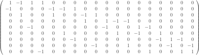
 , where V is the set of vertices and E a set of ordered pairs of distinct vertices representing the edges, and, for each edge an “orientation”. Simply put, an orientation on $\latex \Gamma$ is a list
  of length |E| consisting of
  ‘s. If an edge e=(v,w) is associated to a -1 then we think of the edge as going from w to v; otherwise, it goes from v to w.
 and let
  . The incidence matrix may be regarded as a mapping B from the vector space of function on V to the vector space of functions on E:
 ,
, with the vector space of column vectors
  and
and  with the vector space of column vectors
  then B may be regarded as an
  matrix.
 ,
, ![{\mathbb{Z}}[V]](https://s0.wp.com/latex.php?latex=%7B%5Cmathbb%7BZ%7D%7D%5BV%5D&bg=ffffff&fg=323232&s=0&c=20201002) .
. and
and  are linearly equivalent and write
  if
if  is a principal divisor, i.e., if
 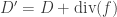 for some function
  . Note that if
 ![[D]](https://s0.wp.com/latex.php?latex=%5BD%5D&bg=ffffff&fg=323232&s=0&c=20201002) the element of the Jacobian determined by
the element of the Jacobian determined by  for all vertices
  to mean that
 is the set of all effective divisors linearly equivalent to
  , then
  . We note also that if
  , then


 according to any proposed reference matrix of the general type described in Section 7, whatever the finite field in which the operations are effected. Such machines would enable us to dispense entirely with tables of any sort, and checks could be determined with great speed. But before checking machines could be seriously planned, the following problem — which is one, incidentally, of considerable interest from the standpoint of pure number theory — would require solution:
 -element sequence
  , a reference matrix
 is the greatest possible. Corresponding to any
 being elements of any given finite algebraic field
  with
with  — determinants of first order (
 ) being single elements of the matrix.
 ,
,  is an
is an  element operand
 -element check based upon the matrix
  is:
is:
 ,
,  .
. ,
,  be a
be a  , \dots, $f_{s}$, $s\leq n$. Let
  . If, in the transmittal of the sequence
 -in-
-in- chance of escaping disclosure, according as $v$ is, or is not, less than
  . In this statement,
  . The presence of error is evidently certain to be disclosed.
 . There is no loss of generality of we assume [This assumption implies
  . – wdj] the $v$ errors are
  ,
,  , affecting
  . The errors cannot escape disclosure. For, to do so, they would have to satisfy the system of homogeneous linear equations:
 contains no vanishing determinant of any order, and which, therefore admits no solution other than
  (
( ).
). errors fall among the
  and
and  errors fall among the
  . Without loss in generality, we may assume that the errors are
  , affecting
  , and
, and  ,
,  , affecting
  ,
,  .
. . Writing
  , where
  denotes a non-negative integer which may or may not be zero, we have
  . Hence
  of the
 denote a set of
  . But the matrix of coefficients in this system contains no vanishing determinant, so that the only solution would be
  ).
). . Then
 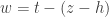 , where $h$ denotes a positive integer. Assuming that the presence of error is to escape detection, we see, therefore, that the
  ) a system of
  equations involving only the errors
  , (
, ( ) a system of
  equations involving all
  — as polynomial functions of the
  errors are determined as rational functions of the remaining
  errors determine the other $t$ errors.
You must be logged in to post a comment.