<a href="m_12.htm#Stabilizer in M24 of a dodecad”>Stabilizer in M24 of a dodecad
1. Mongean Shuffle
The Mongean shuffle concerns a deck of twelve cards, labeled 0 through 11. The permutation
r(t) = 11-t
reverses the cards around. The permutation
s(t) = min(2t,23-2t)
is called the Mongean Shuffle. The permutation group M12 is generated by r and s: M12 = < r,s >, as a subgroup of S12. (See [12], Chap. 11, Sec. 17 or [18])
2. Steiner Hexad
| Jacob Steiner (1796-1863) was a Swiss mathematician specializing in projective goemetry. (It is said that he did not learn to read or write until the age of 14 and only started attending school at the age of 18.) The origins of “Steiner systems” are rooted in problems of plane geometry. |
Let T be a given set with n elements. Then the Steiner system S(k,m,n) is a collection S = {S1, … ,Sr} of subsets of T such that
- |Si| = m,
- For any subset R in T with |R| = k there is a unique i, 1<=i<=n such that R is contained in Si. |S(k,m,n)| = (n choose k)/(m choose k).
If any set H has cardinality 6 (respectively 8, 12) then H is called a hexad, (respectively octad, dodecad.)
Let’s look at the Steiner System S(5,6,12) and M12. We want to construct the Steiner system S(5,6,12) using the projective line P1(F11). To define the hexads in the Steiner system, denote
- the projective line over F11 by P1(F11)={inf,0,1,…,10}.
- Q = {0,1,3,4,5,9}=the quadratic residues union 0
- G = PSL2(F11)
- S = set of all images of Q under G. (Each element g in G will send Q to a subset of P1(F11). )
There are always six elements in such a hexad. There are 132 such hexads. If I know five of the elements in a hexad of S, then the sixth element is uniquely determined. Therefore S is a Steiner system of type (5,6,12).
Theorem:
M12 sends a hexad in a Steiner system to another hexad in a Steiner system. In fact, the automorphism group of a Steiner system of type (5,6,12) is isomorphic to M12.
(For a proof, see [11], Theorem 9.78.)
The hexads of S form a Steiner system of type (5,6,12), so
M12 = < g in S12 | g(s) belongs to S, for all s in S > .
In other words, M12 is the subgroup stabilizing S. The hexads support the weight six words of the Golay code, defined next. (For a proof, see [6].)
3. Golay Code
| ” The Golay code is probably the most important of all codes for both practical and theoretical reasons.” ([17], pg. 64)
M. J. E. Golay (1902-1989) was a Swiss physicist known for his work in infrared spectroscopy among other things. He was one of the founding fathers of coding theory, discovering GC24 in 1949 and GC12 in 1954. |
A code C is a vector subspace of (Fq)n for some n >=1 and some prime power q =pk.
An automorphism of C is a vector space isomorphism, f:C–>C.
If w is a code word in Fqn, n>1, then the number of non-zero coordinates of w is called the weight w, denoted by wt(w). A cyclic code is a code which has the property that whenever (c0,c1,…,cn-1) is a code word then so is (cn-1,c0,…,cn-2).
If c=(c0,c1,…,cn-1) is a code word in a cyclic code C then we can associate to it a polynomial g_c(x)=c0 + c1x + … + cn-1xn-1. It turns out that there is a unique monic polynomial with coefficients in Fq
of degree >1 which divides all such polynomials g_c(x). This polynomial is called
a generator polynomial for C, denoted g(x).
Let n be a positive integer relatively prime to q and let alpha be a primitive n-th root of unity. Each generator g of a cyclic code C of length n has a factorization of the form g(x) = (x-alphak1)… (x-alphakr), where {k1,…,kr} are in {0,…,n-1} [17]. The numbers alphaki, 1≤ i≤ r, are called the zeros of the code C.
If p and n are distinct primes and p is a square mod n, then the quadratic residue code of length n over Fp is the cyclic code whose generator polynomial has zeros
{alphak | k is a square mod n} [17]. The ternary Golary code GC11 is the quadratic
residue code of length 11 over F3.
The ternary Golay code GC12 is the quadratic residue code of length 12 over F3 obtained by appending onto GC11 a zero-sum check digit [12].
Theorem:
There is a normal subgroup N of Aut(GC12) of order 2 such that Aut(GC12)/N is isomorphic to M12. M12 is a quotient of Aut(GC12) by a subgroup or order 2. In other words, M12 fits into the following short exact sequence:
1–>N–>Aut(GC12)–>M12–>1
Where i is the embedding and N in Aut(GC12) is a subgroup of order 2. See [6].
4. Hadamard Matrices
| Jacques Hadamard (1865-1963) was a French mathematician who did important work in analytic number theory. He also wrote a popular book “The psychology in invention in the mathematical field” (1945). |
A Hadamard matrix is any n x n matrix with a +1 or -1 in every entry such that the absolute value of the determinant is equal to nn/2.
An example of a Hadamard matrix is the Paley-Hadamard matrix. Let p be a prime of the form 4N-1, p > 3. A Paley-Hadamard matrix has order p+1 and has only +1’s and -1’s as entries. The columns and rows are indexed as (inf,0,1,2,…,p-1). The infinity row and the infinity column are all +1’s. The zero row is -1 at the 0th column and at the columns that are quadratic non-residues mod p; the zero row is +1 elsewhere. The remaining p-1 rows are cyclic shifts of the finite part of the second row. For further details, see for example [14].
When p = 11 this construction yields a 12×12 Hadamard matrix.
Given two Hadamard Matrices A, B we call them left-equivalent if there is an nxn signed permutation matrix P such that PA = B.
The set {P nxn signed permutation matrix| AP is left equivalent to A} is called the automorphism group of A. In other words, a matrix is an automorphism of the Hadamard matrix, if it is a nxn monomial matrix with entries in {0,+1,-1} and when it is multiplies the Hadamard matrix on the right, only the rows may be permuted, with a sign change in some rows allowed.
Two nxn Hadamard matrices A, B are called equivalent if there are nxn signed permutation matrices P1, P2 such that A = P1 *B *P2.
All 12×12 Hadamard matrices are equivalent ([13], [16] pg. 24). The group of automorphisms of any 12×12 Hadamard matrix is isomorphic to the Mathieu group M12 ([14] pg 99).
5. 5-Transitivity
| Emile Mathieu (1835-1890) was a mathematical physicist known for his solution to the vibrations of an elliptical membrane. |
The fact that M12 acts 5-transitively on a set with 12 elements is due to E. Mathieu who proved the result in 1861. (Some history may be found in [15].)
There are only a finite number of types of 5-transitive groups, namely Sn (n>=5), An (n>=7), M12 and M24. (For a proof, see [11])
Let G act on a set X via phi : G–>SX. G is k-transitive if for each pair of ordered k-tuples (x1, x2,…,xk), (y1,y2,…,yk), all xi and yi elements belonging to X, there exists a g in G such that yi = phi(g)(xi) for each i in {1,2,…,k}.
M12 can also be constructed as in Rotman [11], using transitive extensions, as follows (this construction appears to be due originally to Witt). Let fa,b,c,d(x)=(ax+b)/(cx+d), let
M10 = < fa,b,c,d, fa’,b’,c’,d’ |ad-bc is in Fqx, a’d’-b’c’ is not in Fqx >,
q = 9.
pi = generator of F9x, so that F9x = < pi> = C8.
Using Thm. 9.51 from Rotman, we can create a transitive extension of M10. Let omega be a new symbol and define
M11 = < M10, h| h = (inf, omega)(pi, pi2)(pi3,pi7) (pi5,pi6)>.
Let P1(F9) = {inf, 0, 1, pi, pi2, … , pi7}. Then M11 is four transitive on Y0 = P1(F9) union {omega}, by Thm 9.51.
Again using Thm. 9.51, we can create a transitive extension of M11. Let sigma be a new symbol and define
M12 = < M11, k>, where k = (omega, sig)(pi,pi3) (pi2,pi6)(pi5,pi7). M12 is 5-transitive on Y1 = Y0 union {sig}, by Th. 9.51.
Now that we constructed a particular group that is 5-transitive on a particular set with 12 elements, what happens if we have a group that is isomorphic to that group? Is this new group also 5-transitive?
Let G be a subgroup of S12 isomorphic to the Mathieu group M12. Such a group was constructed in Section 1.
Lemma: There is an action of G on the set {1,2,…,12} which is 5-transitive.
proof: Let Sig : G –> M12 be an isomorphism. Define g(i) = Sig(g)(i), where i = {1,2,…,12}, g is in G. This is an action since Sig is an isomorphism. Sig-1(h)(i) = h(i) for all g in M12, i in Y1. Using some h in M12, any i1,…,i5
in Y1 can be sent to any j1,…,j5 in Y1. That is, there exists an h in M12 such that h(ik) = jk, k= 1,…,5 since M12 is 5-transitive. Therefore, Sig-1(h)(ik) = jk = g(ik). This action is 5-transitive. QED
In fact, the following uniqueness result holds.
Theorem: If G and G’ are subgroups of S12 isomorphic to M12 then they are conjugate in S12.
(This may be found in [7], pg 211.)
6. Presentations
The presentation of M12 will be shown later, but first I will define a presentation.
Let G = < x1,…,xn | R1(x1,…xn) = 1, …, Rm(x1,…,xn) = 1> be the smallest group generated by x1,…,xn satisfying the relations R1,…Rm. Then we say G has presentation with generators x1,…,xn and relations R1(x1,…xn) = 1, …, Rm(x1,…,xn) = 1.
Example: Let a = (1,2,…,n), so a is an n-cycle. Let Cn be the cyclic group, Cn = < a > =
{1,a,…,an-1}. Then Cn has presentation < x | xn=1 > = all words in x, where x satisfies xn.=1 In fact, < x | xn = 1 > is isomorphic to < a >. Indeed, the isomorphism
< x | xn = 1 > –> < a > is denoted by xk –> ak, 0 <= k <= n-1. Two things are needed for a presentation:
- generators, in this case x, and
- relations, in this case xn = 1.
Example: Let G be a group generated by a,b with the following relations; a2 = 1, b2 = 1, (ab)2 = 1:
G = < a,b | a2 = 1, b2 = 1, (ab)2 = 1 > = {1,a,b,ab}.
This is a non-cyclic group of order 4.
Two presentations of M12 are as follows:
M12 = < A,B,C,D | A11 = B5 = C2 = D2 = (BC)2 = (BD)2 = (AC)3 = (AD)3 = (DCB)2 = 1, AB =A3 >
= < A,C,D | A11 = C2 = D2 = (AC)3 = (AD)3 = (CD)10 = 1, A2(CD)2A = (CD)2 >.
In the first presentation above, AB = B-1AB. These are found in [6] and Chap. 10 Sec. 1.6 [12].
7. Crossing the Rubicon
The Rubicon is the nick-name for the Rubik icosahedron, made by slicing the icosahedron in half for each pair of antipodal vertices. Each vertex can be rotated by 2*pi/5 radians, affecting the vertices in that half of the Rubicon, creating a shape with 12 vertices, and six slices. The Rubicon and M12 are closely related by specific moves on the Rubicon.
Let f1, f2, …,f12 denote the basic moves of the Rubicon, or a 2*pi/5 radians turn of the sub-pentagon about each vertex. Then according to Conway,
M12 = < x*y-1 | x,y are elements of {f1, f2, …,f12 } >.
Actually, if a twist-untwist move, x*y-1, as above, is called a cross of the Rubicon, then M12 is generated by the crosses of the Rubicon! ([1], Chap. 11 Sec. 19 of [12])
<a name="M12 and the Minimog”>
8. M12 and the Minimog
Using the Minimog and C4 (defined below), I want to construct the Golay code GC12.
The tetracode C4 consists of 9 words over F3:
  0 000,     0 +++,    0 ---,         where 0=0, +=1, and -=2 all mod 3.
  + 0+-,     + +-0,    + -0+,
  - 0-+,     - +0-,    - -+0.
Each (a,b,c,d) in C4 defines a linear function f : F3 –> F3, where f(x) = ax+b, f(0) = b, f(1) = f(+) = c, f(2) = f(-) = d, and a is the “slope” of f. This implies a + b = c (mod 3), b – a = d (mod 3).
Minimog: A 4×3 array whose rows are labeled 0,+,-, that construct the Golay code in such a way that both signed and unsigned hexads are easily recognized.
A col is a word of length 12, weight 3 with a “+” in all entries of any one column and a “0” everywhere else. A tet is a word of length 12, weight 4 who has “+” entries in a pattern such that the row names form a tetracode word, and “0” entires elsewhere. For example,
             _________          _________
             | |+    |          | |+    |
             | |+    |          |+|  +  |
             | |+    |          | |    +|
             ---------          ---------
             "col"              "tet"
The above “col” has “+” entries in all entries of column 2, and “0” entries elsewhere.
The above “tet” has a “+” entry in each column. The row names of each “+” entry are +, 1, +, – respectively. When put together, + 0+- is one of the nine tetracode words.
Lemma: Each word belongs to the ternary Golay Code GC12 if and only if
- sum of each column = -(sum row0)
- row+ – row – is one of the tetracode words.
This may be found in [4].
Example:
|+|+ + +|      col sums: ----      row+ - row-: --+0
|0|0 + -|      row0 sum: + = -(sum of each col)
|+|+ 0 -|
How do I construct a Golay code word using cols and tets? By the Lemma above, there are four such combinations of cols and tets that are Golay code words. These are: col – col, col + tet, tet – tet, col + col – tet.
Example:
  col-col         col+tet      tet-tet       col+col-tet

 | |+   -|       | |+ +  |    |+|0 + +|      | |- + +|
 | |+   -|       |+|  -  |    |-|  -  |      |-|  0 +|
 | |+   -|       | |  + +|    | |    -|      | |  + 0|
  ? ? ? ?         + 0 ? -      - ? - +        + 0 + -
“Odd-Man-Out”: The rows are labeled 0,+,-, resp.. If there is only one entry in a column then the label of the corresponding row is the Odd Man Out. (The name of the odd man out is that of the corresponding row.) If there is no entry or more than one entry in the column then the odd man out is denoted by “?”.
For example, in the arrays above, the Odd-Men-Out are written below the individual arrays.
For the Steiner system S(5,6,12), the minimog is labeled as such:
                              ______________
                              |0  3 inf  2 |
                              |5  9  8  10 |
                              |4  1  6  7  |
                              --------------
The four combinations of cols and tets above that construct a Golay code word yield all signed hexads. From these signed hexads, if you ignore the sign, there are 132 hexads of the Steiner system S(5,6,12) using the (o, inf, 1) labeling discussed in Section 9 below. There are a total of 265 words of this form, but there are 729 Golay code words total. So, although the above combinations yield all signed hexads, they do not yield all hexads of the Golay code ([12] pg. 321).
The hexad for the tet-tet according to the S(5,6,12) Minimog above would be (0, inf, 2, 5, 8, 7).
The rules to obtain each hexad in this Steiner system is discussed in Section 9 below.
A Steiner system of type (5,6,12) and the Conway-Curtis notation can be obtained from the Minimog. S12 sends the 3×4 minimog array to another 3×4 array. The group M12 is a subgroup of S12 which sends the Minimog array to another array also yielding S(5,6,12) in Conway-Curtis notation.
9. Kitten
The kitten is also an interesting facet of the Minimog. Created by R.T. Curtis,
kittens come from the construction of the Miracle Octal Generator, or MOG, also created by R.T. Curtis. (A description of the MOG would be too far afield for this post, but further information on the MOG can be gotten from [3] or [6].)
Suppose we want to construct a Steiner system from the set T = {0, 1, …, 10, inf}.
The kitten places 0, 1, and inf at the corners of a triangle, and then creates a rotational symmetry of triples inside the triangle according to R(y) = 1/(1-y) (as in [2], section 3.1). A kitten looks like:
                                infinity

                                   6

                                2     10

                             5     7      3

                          6     9      4     6

                       2    10     8      2     10

                 0                                    1

                            Curtis' kitten
where 0, 1, inf are the points at infinity.
Another kitten, used to construct a Steiner system from the set T = {0, 1, …, 10, 11} is
                                   6

                                   9

                                10     8

                             7     2      5

                          9     4     11     9

                      10     8     3      10     8

                 1                                    0

                         Conway-Curtis' kitten
The corresponding minimog is
                  _________________________
                  |  6  |  3  |  0  |  9  |
                  |-----|-----|-----|-----|
                  |  5  |  2  |  7  | 10  |
                  |-----|-----|-----|-----|
                  |  4  |  1  |  8  | 11  |
                  |_____|_____|_____|_____|
(see Conway [3]).
The first kitten shown consists of the three points at 0, inf, 1 with an arrangement of points of the plane corresponding to each of them. This correspondence is:
         6 |10 | 3              5 | 7 |3               5 | 7 | 3
         2 | 7 | 4              6 | 9 |4               9 | 4 | 6
         5 | 9 | 8              2 |10 |8               8 | 2 |10

        inf-picture             0-picture              1-picture
A union of two perpendicular lines is called a cross. There are 18 crosses of the kitten:
                ___________________________________________
                |* * * |* * * |* * * |*     |  *   |    * |
                |*     |  *   |    * |* * * |* * * |* * * |
                |*     |  *   |    * |*     |  *   |    * |
                 -----------------------------------------
                 _________________________________________
                |*     |  *   |* *   |*     |*   * |    * |
                |*     |  *   |* *   |  * * |  *   |    * |
                |* * * |* * * |    * |  * * |*   * |* * * |
                 -----------------------------------------
                 _________________________________________
                |*   * |    * |  * * |  *   |  * * |* *   |
                |*   * |* *   |*     |*   * |  * * |    * |
                |  *   |* *   |  * * |*   * |*     |* *   |
                ------------------------------------------
A square is a complement of a cross. The 18 squares of a kitten are:
                ___________________________________________
                |      |      |      |  * * |*   * |* *  |
                |  * * |*   * |* *   |      |      |     |
                |  * * |*   * |* *   |* *   |*   * |* *  |
                 -----------------------------------------
                 _________________________________________
                |  * * |*   * |    * |  * * |  *   |* *   |
                |  * * |*   * |    * |*     | *  * |* *   |
                |      |      |* *   |*     |  *   |      |
                 -----------------------------------------
                 _________________________________________
                |  *   |* *   |*     |*   * |*     |    * |
                |  *   |    * |  * * |  *   |*     |* *   |
                |*   * |    * |*     |  *   |  * * |    * |
                 -----------------------------------------
The rules to obtain a hexad in the {0,1,inf} notation are the following:
- A union of parallel lines in any picture,
- {0, 1, inf} union any line,
- {Two points at infinity} union {square in a picture corresponding to omitted point at infinity},
- {One point at infinity} union {cross in the corresponding picture at infinity}.
(See [2])
M12 is isomorphic to the group of automorphisms of the Steiner system S(5,6,12) in the Conway-Curtis notation.
10. Mathematical Blackjack or Mathieu’s 21
Mathematical Blackjack is a card game where six cards from the group {0,1,…,11} are laid out face up on a table. The rules are:
- each player must swap a card with a card from the remaining six, that is lower than the card on the table;
- the first player to make the sum of all six cards less than 21 loses.
According to Conway and Ryba [8, section V, part (d)], the winning strategy of this game is to choose a move which leaves a Steiner hexad from S(5,6,12) in the shuffle
notation, whose sum is greater than or equal to 21, on the table.
The shuffle notation for the hexad, used in the Mathematical Blackjack game, is shown below (see also the description in the hexad/blackjack page):
              8 |10 |3            5 |11 |3            5 |11 |3
              9 |11 |4            2 | 4 |8            8 | 2 |4
              5 | 2 |7            7 | 9 |10           9 |10 |7

             0-picture          1-picture          6-picture
Riddle: Assuming the strategy, player A just made a winning hexad move that will force player B to make the sum under 21 on his next turn. Joe Smith walks up to player B and offers to shuffle all 12 cards while player A isn’t looking, for a fee. Player B grabs at his chance thinking that a random shuffle will let him back in the game. How is it that player B still loses?
Joe is actually working for Player A. Joe does not shuffle the cards randomly, but instead uses the M12 group generated by r, s (see section 1) to shuffle the cards. Since the M12 group preserves hexads, player A still has a winning game. (He and Joe split the money.)
11. Sporadic Groups
A simple group is a group with no normal subgroups except itself and {1}. Most simple groups are from a family such as PSL2(Fp), p>3 or An, n >= 5. However there exist some simple groups outside of such well known families. These are called sporadic simple groups. M12 is a sporadic simple group of order 95,040. The only smaller sporadic group is M11 of order 7,920. (See [10] pg. 211)
<a name="Stabilizer in M24 of a dodecad”>
12. Stabilizer in M24 of a dodecad.
M24 is a sporadic simple group of order 244,823,040 containing M12 as a subgroup. The Steiner system S(5,8,24) is a collection of 8 element subsets, called octads, from a 24 element set X, with the property that any five elements in X determine a unique octad in the system. There are (24 choose 5)/(8 choose 5) = 759 of these octads. M24 is the subgroup of SX which sends the set of octads to itself. Two octads, O1, O2, intersect in a subset of X of order 0,2,4,6 or 8 [14]. If |O1 intersect O2| = 2 then O1 + O2 is order 12. Such a subset of X is called a dodecad. M12 is isomorphic to
{g in M24 | g(O1 + O2) = (O1 + O2)} = the stablizer of the dodecad O1 + O2.
(See [6] for details)
Much more information can be received from the references below or from the hexad/blackjack page.
References
- W. D. Joyner, Mathematics of the Rubik’s Cube (USNA Course notes), 1997.
- R. T. Curtis, “The Steiner System S(5,6,12), the Mathieu Group M12 and the ‘Kitten’ ,” Computational Group Theory, Academic Press, London, 1984.
- J. H. Conway, “hexacode and Tetracode- MOG and MINIMOG,” Computational Group Theory (ed. Atkinson), Academic Press, London, 1984.
- Vera Pless, “Decoding the Golay Code,” Transactions of Information Theory, IEEE, 1986, (pgs 561-567).
- R. T. Curtis, “A new Combinatorial approach to M24“, Mathematical Proceeding of the Cambridge Philosophical Society, Vol. 79, 1974.
- J. H. Conway, R. T. Curtis, S. P. Norton, R. A. Parker, R. A. Wilson, “M12,”,
Atlas of Finite Groups, Clarendon Press, Oxford, 1985.
- Robinson, A Course in the Theory of Groups, Springer, 1996.
- J. H. Conway, N. Sloane, “Lexicographic Codes: Error-Correcting Codes
from Game Theory,” Transactions on Information Theory, IEEE, 1986.
- A .Adler, “The modular Curve X(11) and the Mathieu group M11“,
Proc. London Math Society 74(1997)1-28.
See also the paper X(11) and M11.
- T. Thompson, From Error-Correcting Codes Through Sphere
Packings to Simple Groups, The Mathematical Association of
America, 1983.
- Rotman, J, Introduction to the Theory of Groups, 4th ed.
Springer-Verlag, 1995.
- J. Conway, N. Sloane, Sphere Packings, Lattices, and Groups,
Springer-Verlag, 3rd ed., 1999.
- B. Kostant, “The Graph of the truncated icosahedron and the
last letter of Galois.” Notices of the A.M.S. 42(1995)959-
968.
- E. Assmus, “On the Automorphism Groups of Paley-Hadamard
Matrices.” Combinatorial Mathematics and its Applications.
University of North Carolina Press, 1969, (pgs 98-103).
- P. Greenberg, Mathieu Groups, Courant Institute of Math and
Science, New York University, 1973.
- P. Cameron, J. Van Lint, Designs, Graphs, Codes, and Their
Links, London Mathematical Society, Cambridge University
Press, 1991.
- F. MacWilliams, N. Sloane, The Theory of Error Correcting
Codes, North Holland Publishing Company, 1978.
- R. Graham, P. Diaconis, W. Kantor, “The Mathematics of
Perfect Shuffles”, Advanced Applied Math, Vol. 4, 1985, (pgs
175-196).
Typed into html by wdj, 4-18-97.
Corrections 4-27-2001.
Last updated 2018-06-10.


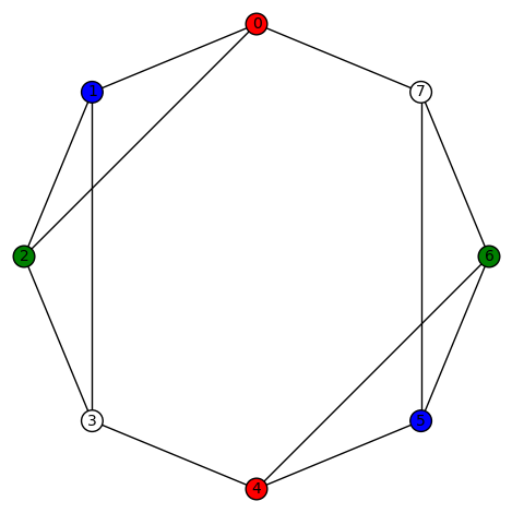
. This graph is not vertex transitive. Its characteristic polynomial is
. Its edge connectivity and vertex connectivity are both 2. This graph has no non-trivial harmonic morphisms to D3 or P4 or C4 or Paw. However, there are 48 non-trivial harmonic morphisms to
. For example,
 (the automorphism group of K4, ie the symmetric group of degree 4, acts on the colors {0,1,2,3} and produces 24 total plots), and
  (again, the automorphism group of K4, ie the symmetric group of degree 4, acts on the colors {0,1,2,3} and produces 24 total plots). There are 8 non-trivial harmonic morphisms to
 . For example,
 and
and  Here the automorphism group of K4, ie the symmetric group of degree 4, acts on the colors {0,1,2,3}, while the automorphism group of the graph
 (obviously too small to act transitively on the vertices). Its characteristic polynomial is
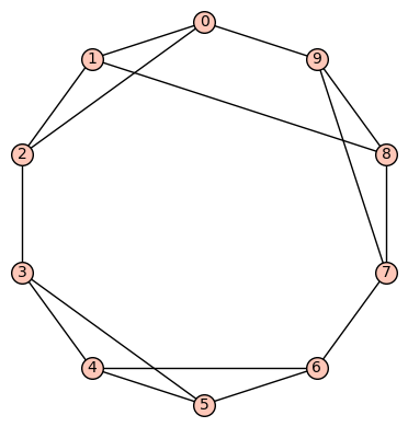
, its edge connectivity and vertex connectivity are both 3. This graph has no non-trivial harmonic morphisms to D3 or P4 or C4 or Paw or K4. However, it has 4 non-trivial harmonic morphisms to Diamond. They are:


 Let
Let . It does not act transitively on the vertices. Its characteristic polynomial is
and its edge connectivity and vertex connectivity are both 3.
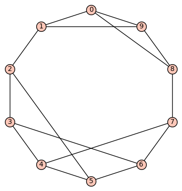
, this graph
. It is vertex transitive. Its characteristic polynomial is
and its edge connectivity and vertex connectivity are both 3.
 A few examples of a non-trivial harmonic morphism to Diamond:
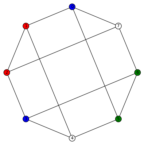 and
and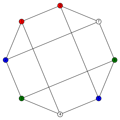 A few examples of a non-trivial harmonic morphism to C4:


 be an
be an ![[n,k,d]_q](https://s0.wp.com/latex.php?latex=%5Bn%2Ck%2Cd%5D_q&bg=ffffff&fg=323232&s=0&c=20201002) code, ie a linear code over
code, ie a linear code over  of length
  , dimension
  , and minimum distance
  . In general, if
 ![[n,k^\perp,d^\perp]_q](https://s0.wp.com/latex.php?latex=%5Bn%2Ck%5E%5Cperp%2Cd%5E%5Cperp%5D_q&bg=ffffff&fg=323232&s=0&c=20201002) for the parameters of the dual code,
for the parameters of the dual code,  . It is a consequence of Singleton’s bound that
  , with equality when
  :
:
 is a polynomial of degree
  , called the zeta polynomial of
 ![[n,n-k,d^\perp]](https://s0.wp.com/latex.php?latex=%5Bn%2Cn-k%2Cd%5E%5Cperp%5D&bg=ffffff&fg=323232&s=0&c=20201002) then the MacWilliams identity relates the weight enumerator
then the MacWilliams identity relates the weight enumerator  of
of  of
of 

 and
and  then the Duursma zeta polynomial
  exists and is unique.
 be a graph having
  vertices and
  edges. We define the zeta function of
  via the Duursma zeta function of the binary linear code defined by the cycle space of
  generated by the rows of the incidence matrix of
  , and the dual code
  is the cycle space
  of
of 
 is
is  , dimension of
  , and the minimum distance of
  is
is  , and the minimum distance of
 is the Duursma polynomial of
  , the wheel graph on 5 vertices, we have
 .
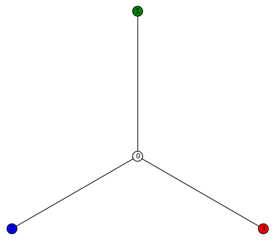
. . This graph is also called a star graph
  on 3+1=4 vertices, or the bipartite graph
  .
.
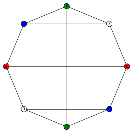
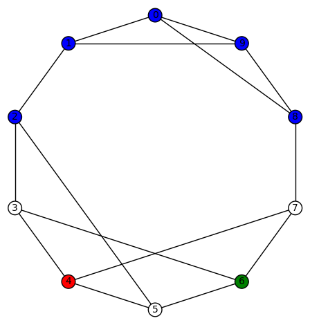
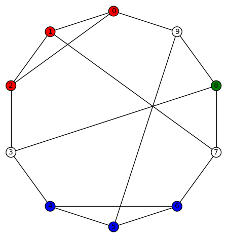
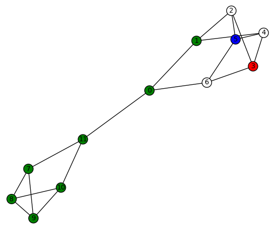
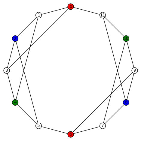
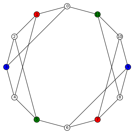
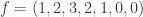
 sends the red vertices in
  is a harmonic morphism. Let
  be adjacent vertices of
  and
and  or (b)
  and the vertices
  and
and  are adjacent in
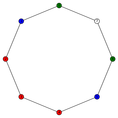
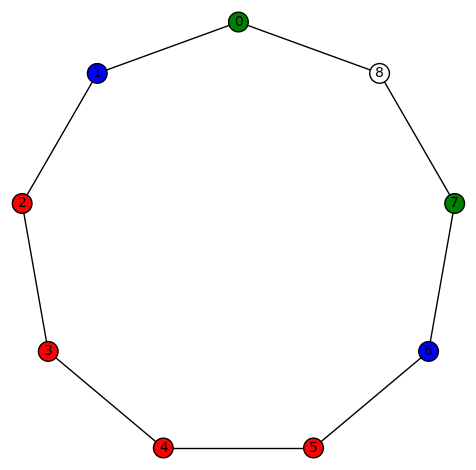
  the green vertex is not adjacent to the blue or red vertex, none of the harmonic colored graphs below can have a green vertex adjacent to a blue or red vertex. In fact, any colored vertex can only be connected to a white vertex or a vertex of like color.
 , plus the “obvious” ones obtained from that below and those induced by permutations of the vertices:
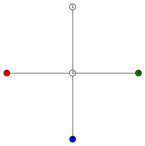 .
.  can be described in a similar manner. Likewise for the higher
  graphs. Given a star graph

 , plus the “obvious” ones obtained from that above and those induced by permutations of the vertices with a non-zero color.
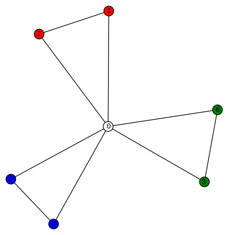
 , one hovering over the other. Now, connect each vertex of the top copy to the corresponding vertex of the bottom copy. This is a cubic graph that can be visualized as a “thick” regular polygon. (The cube graph is the case
  .) I conjecture that there is no harmonic morphism from such a graph to
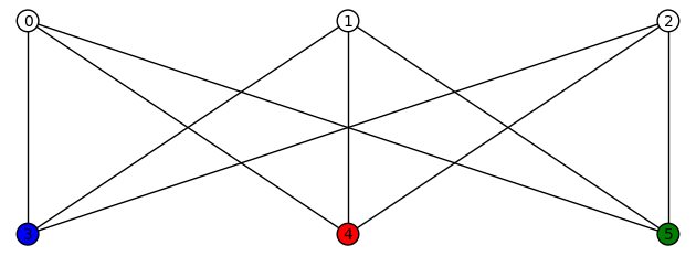
 for the complete bipartite (“utility”) graph
  . They are all obtained from either
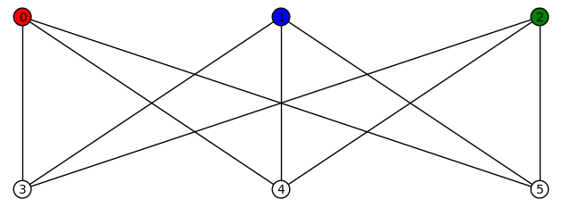
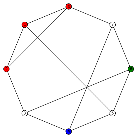
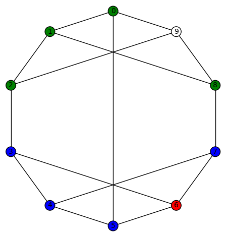
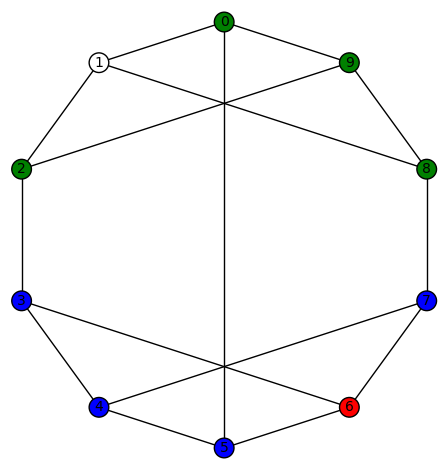
 , where
  and
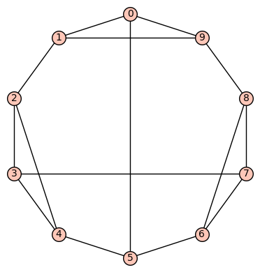
and  . This graph has diameter 3, girth 3, and edge-connectivity 3. It’s automorphism group is size 4, generated by (5,9) and (1,8)(2,7)(3,6). The harmonic morphisms are all obtained from
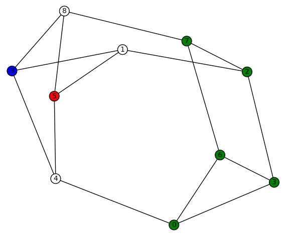


 .
.


 , where
  .
. .
. .
.

 .
. . (This only differs by one edge from the one above.)

 .
. .
.


 . Denote the
  . We write an element of this space as
  , where the variables
  will be called coordinate variables. Let
 . In this post, the cosets
 ). A function in
  which (a) is constant along some coordinate hyperplane
  , (b) whose restriction
  is constant along some coordinate hyperplane
  , (c) whose restriction
  is constant along some coordinate hyperplane
  , (d) and so on. This “nested” inductive definition might seem complicated, but to a computer it’s pretty simple and, to boot, it requires little memory to store.
  and
and  then let
  denote the vector whose i-th coordinate is flipped (bitwise). The sensitivity of
  is
is . Roughly speaking, it’s the number of single-bit changes in
  . The (maximum) sensitivity is the quantity
 The block sensitivity is defined similarly, but you allow blocks of indices of coordinates to by flipped bitwise, as opposed to only one. It’s possible to
  .
.
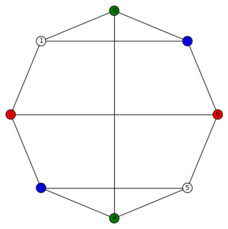
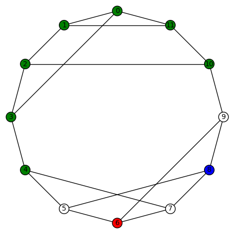
 the white vertex is not adjacent to the blue or red vertex, none of the harmonic colored graphs below can have a white vertex adjacent to a blue or red vertex.
 as the domain in this post. However, before we get to examples (obtained by using
 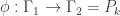 be a harmonic morphism from a graph
  vertices to the path graph having
  vertices. Let
  be the coloring map (identified with an n-tuple whose coordinates are in
  ). Associated to f is a partition
 ![\Pi_f=[n_0,\dots,n_{k-1}]](https://s0.wp.com/latex.php?latex=%5CPi_f%3D%5Bn_0%2C%5Cdots%2Cn_%7Bk-1%7D%5D&bg=ffffff&fg=323232&s=0&c=20201002) of n (here
of n (here ![[...]](https://s0.wp.com/latex.php?latex=%5B...%5D&bg=ffffff&fg=323232&s=0&c=20201002) is a multi-set, so repetition is allowed but the ordering is unimportant):
is a multi-set, so repetition is allowed but the ordering is unimportant):  , where
  is the number of times j occurs in f. We call this the partition invariant of the harmonic morphism.
  ,
,  , with associated
 whose corresponding partitions agree,
  then we say
  and
and  are partition equivalent.
 examples!
 , so we start with
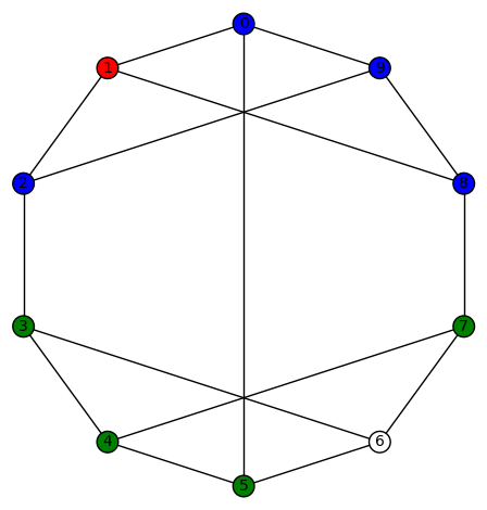
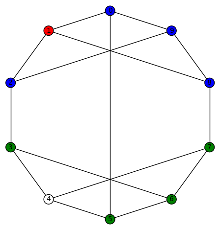
  . We indicate a harmonic morphism by a vertex coloring. An example of a harmonic morphism can be described in the plot below as follows:
  sends the red vertices in
  , plus that induced by
  and all of its cyclic permutations (4+6=10). This set of 6 permutations is closed under the automorphism of
 and all of its cyclic permutations (4+7=11). This set of 7 permutations is not closed under the automorphism of
  and all 7 of its cyclic permutations (total = 7+11 = 18).
 and all of its cyclic permutations (4+8=12). This set of 8 permutations is not closed under the automorphism of
  and all of its cyclic permutations (12+8=20). In addition, there is
  and all of its cyclic permutations (20+8 = 28). The latter set of 8 cyclic permutations of
  is closed under the transposition (0,3)(1,2) (total = 28).

 and all of its cyclic permutations (4+9=13). This set of 9 permutations is not closed under the automorphism of
  and all 9 of its cyclic permutations (9+13 = 22). This set of 9 permutations is not closed under the automorphism of
  and all 9 of its cyclic permutations (9+22 = 31). This set of 9 permutations is not closed under the automorphism of
  and all 9 of its cyclic permutations (total = 9+31 = 40).


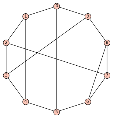
 is the graph whose SageMath command is


 then, instead of showing a graph, I’ll list the edges (of course, the vertices are 0,1,…,11) and the SageMath command for it.
 .
. such that two successive terms differ in only one position. A Gray code can be regarded as a Hamiltonian path in the cube graph. For example:

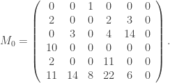
 (regarded as a weighted adjacency matrix) is in the figure below.
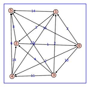

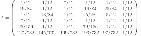
 by
by  , where
  is the
  doubly stochastic matrix with every entry equal to
  :
:

 associated to the largest eigenvalue
  (by reverse, I mean that the vector ranks the teams from worst-to-best, not from best-to-worst, as we have seen in previous ranking methods).

 Lafayette
  .
.
You must be logged in to post a comment.