TS Michael passed away on November 22, 2016, from cancer. I will miss him as a colleague and a kind, wise soul. Tom Quint has kindly allowed me to post these reminiscences that he wrote up.
Well, I guess I could start with the reason TS and I met in the first place. I was a postdoc at USNA in about 1991 and pretty impressed with myself. So when USNA offered to continue my postdoc for two more years (rather than give me a tenure track position), I turned it down. Smartest move I ever made, because TS got the position and so we got to know each other.
We started working w each other one day when we both attended a talk on “sphere of influence graphs”. I found the subject moderately interesting, but he came into my office all excited, and I couldn’t get rid of him — wouldn’t leave until we had developed a few research ideas.
Interestingly, his position at USNA turned into a tenure track, while mine didn’t. It wasn’t until 1996 that I got my position at U of Nevada.
Work sessions with him always followed the same pattern. As you may or may not know, T.S. a) refused to fly in airplanes, and b) didn’t drive. Living across the country from each other, the only way we could work together face-to-face was: once each summer I would fly out to the east coast to visit my parents, borrow one of their cars for a week, and drive down to Annapolis. First thing we’d do is go to Whole Foods, where he would load up my car with food and other supplies, enough to last at least a few months. My reward was that he always bought me the biggest package of nigiri sushi we could find — not cheap at Whole Foods!
It was fun, even though I had to suffer through eight million stories about the USNA Water Polo Team.
Oh yes, and he used to encourage me to sneak into one of the USNA gyms to work out. We figured that no one would notice if I wore my Nevada sweats (our color is also dark blue, and the pants also had a big “N” on them). It worked.
Truth be told, TS didn’t really have a family of his own, so I think he considered the mids as his family. He cared deeply about them (with bonus points if you were a math major or a water polo player :-).
One more TS anecdote, complete with photo. Specifically, TS was especially thrilled to find out that we had named our firstborn son Theodore Saul Quint. Naturally, TS took to calling him “Little TS”. At any rate, the photo below is of “Big TS” holding “Little TS”, some time in the Fall of 2000.

TS Michael in 2000.
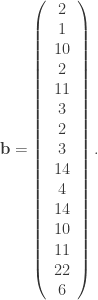
 against team
  is
is  , and the total runs allowed by team
  . Here, we order the six teams as above (team
  is Army (USMI at Westpoint), team
  is Bucknell, and so on). For instance if X played Y and the scores were
  ,
,  ,
,  in the position of row X and column Y.
 matrix:
 which best fits the equation

 with linearly independent columns. Unfortunately, in this case
  does not have linearly independent columns, so the formula doesn’t apply.
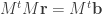


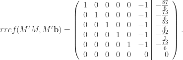
 denotes the rankings of Army, Bucknell, Holy Cross, Lafayette, Lehigh, Navy, in that order, then
 Army = Bucknell = Lehigh
  .
.


 Team
Team  Team
Team  denote some fixed ranking (where
  is some permutation of
  ). An upset occurs when a lower ranked team beats an upper ranked team. For each ranking,
  denote the total number of upsets. The minimum upset problem is to find an “efficient” construction of a ranking for which
  denote the number of times Team i beat team $j$ minus the number of times Team j beat Team i. We regard this matrix as the signed adjacency matrix of a digraph
  . Our goal is to find a Hamiltonian (undirected) path through the vertices of
  , with rows and columns indexed by the teams in some fixed order. The entry in the i-th row and the j-th column is defined by
 , and those that lost the most at the bottom.
 board may be represented graph theoretically as a Hamiltonian cycle on a particular graph with
  vertices, of which
  of them have degree
  ,
,  have degree
  and the remaining
  vertices have degree
  . The problem of finding an algorithm to find a hamiltonian circuit in a general graph is known to be NP complete. The problem of finding an efficient algorithm to search for such a tour therefore appears to be very hard problem. In [BK], C. Bailey and M. Kidwell proved that complete even king tours do not exist. They left the question of the existence of complete odd tours open but showed that if they did exist then it would have to end at the edge of the board.
 and
and  ,
, ,
,  and
and  or
or  (or both) is odd,
 ,
,  and the tour is “rapidly filling”.
 array of neighboring squares on the board. A foursome is called completed if all four squares have been visited by the the king at some point in a tour, including the case where the king is still on one of the four squares.
 denote the change in the number of completed foursomes and let
  denote the change in the number of completed neighbor pairs. Note that

 then
then  . If
. If  then
then  . If
. If  then
then  . If
. If  then
then  .
.  . If
. If  . If
. If  . If
. If  .
.  and
and  .
. denote the total number of completed neighbor pairs after a given point of a given odd king tour. We may represent the values of
  . Here
  is the total number of completed neighbor pairs after the first move,
  . In particular, the parity of
  , which is obviously even. This is a contradiction. QED
 is odd. This follows from a computer computation, an argument from Sands [Sa], and the sequence of lemmas that follow. The proofs are in the original paper, and omitted.
 denote the number of completed foursomes in a given odd king tour. Let $M$ denote the number of moves in a given odd king tour. Let
 , where
  are defined as above. Then
  equals
  ,
,  only occurs when
  .
. denote the largest number of non-overlapping
 ![[m/2][n/2]](https://s0.wp.com/latex.php?latex=%5Bm%2F2%5D%5Bn%2F2%5D&bg=ffffff&fg=323232&s=0&c=20201002) 0’s.
0’s. on an
on an  then all
  boards have nearly complete odd king tours.
 ,
, ![{\mathbb{Z}}[V]](https://s0.wp.com/latex.php?latex=%7B%5Cmathbb%7BZ%7D%7D%5BV%5D&bg=ffffff&fg=323232&s=0&c=20201002) .
. and
and  are linearly equivalent and write
  if
if  is a principal divisor, i.e., if
  for some function
  . Note that if
 ![[D]](https://s0.wp.com/latex.php?latex=%5BD%5D&bg=ffffff&fg=323232&s=0&c=20201002) the element of the Jacobian determined by
the element of the Jacobian determined by  for all vertices
  . We write
  to mean that
 is the set of all effective divisors linearly equivalent to
  , then
  . We note also that if
  , then
  between graphs
  and
and  can be uniquely defined by specifying where the vertices of
  go. If
  and
and  then this is a list of length
  consisting of elements taken from the
  vertices in
  .
. and let
  denote the “cube graph” (actually the unit square) in
  .
.

 by
by to be a subgraph of
  is called harmonic if for all vertices
  , the quantity
 in
in  .
. . In this post, I’d like to give some more examples, based on a
  . The Cayley graph of
 and the set of edges is defined by
 has weight
  . However, if
  as an edge-weighted (undirected) graph.
  , define
 to be the set of all neighbors of
  in
in  to be the set of all neighbors
  ),
),
 to be the set of all non-neighbors
  ),
),

 ,
,  ,
,  , denoted
  , if it consists of

 ,
,  ,
,  are as above. Here,
  is the set of weights, including
  listed in the table below
![GF(9) = GF(3)[x]/(x^2+1) = \{0,1,2,x,x+1,x+2,2x,2x+1,2x+2\}.](https://s0.wp.com/latex.php?latex=GF%289%29+%3D+GF%283%29%5Bx%5D%2F%28x%5E2%2B1%29+%3D+%5C%7B0%2C1%2C2%2Cx%2Cx%2B1%2Cx%2B2%2C2x%2C2x%2B1%2C2x%2B2%5C%7D.++&bg=ffffff&fg=323232&s=0&c=20201002)
 and whose edges
  are those pairs for which
  .
.


 .
.
 be a finite set and let
  denote binary relations on
  ). The dual of a relation
  is the set
 . We say
  is an
is an  -class association scheme on
 for all $i\not= j$.
 (and if
  for all
  and all
  , define

 , the integer
  is a constant, denoted
  .
.
 and
and  of the association scheme
  , where
  ,
, 
 .
.

 is
is 
 is the identity matrix. In the above computation, Sage has also verified that they commute and satisfy
 . If the level curves of
  be a prime power such that
  . Note that this implies that the unique finite field of order
  , has a square root of
  and
and
 if and only if
  . By definition
  is the
  (with multiplicity
  (both with multiplicity
  , where
  is prime, then
  has order
  .
. ” above; I was having trouble rendering it in html.) Below is an example.
 , it has only three distinct eigenvalues, and its automorphism group is order
  .
. :
: :
:
You must be logged in to post a comment.