This post expands on a previous post and gives more examples of harmonic morphisms to the tree 


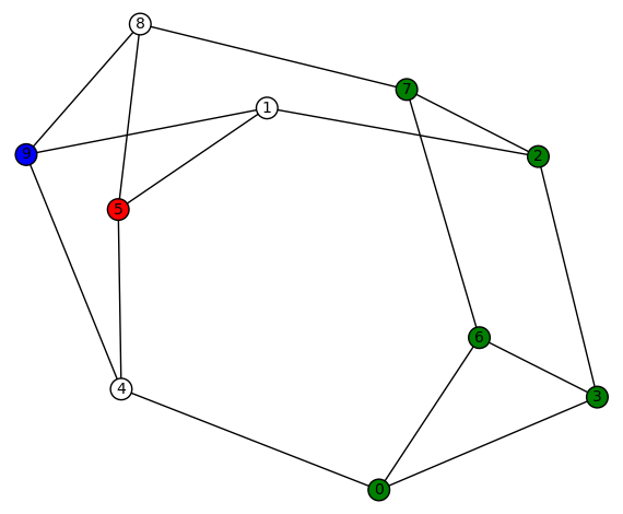
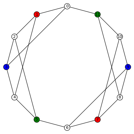
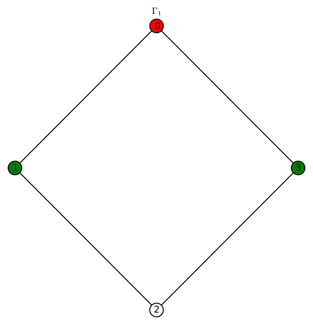
We indicate a harmonic morphism by a vertex coloring. An example of a harmonic morphism can be described in the plot below as follows: 

First, a simple remark about harmonic morphisms in general: roughly speaking, they preserve adjacency. Suppose 


To get the following data, I wrote programs in Python using SageMath.
Example 1: There are only the 4 trivial harmonic morphisms 
 .
.
My guess is that the harmonic morphisms 


Example 2: For graphs like

there are only the 4 trivial harmonic morphisms 

Example 2.5: Likewise, for graphs like

there are only the 4 trivial harmonic morphisms
Example 3: This is really a non-example. There are no harmonic morphisms from the (3-dimensional) cube graph (whose vertices are those of the unit cube) to
More generally, take two copies of a cyclic graph on n vertices, 

Example 4: There are 30 non-trivial harmonic morphisms

Another interesting fact is that this graph has an automorphism group (isomorphic to the symmetric group on 5 letters) which acts transitively on the vertices.
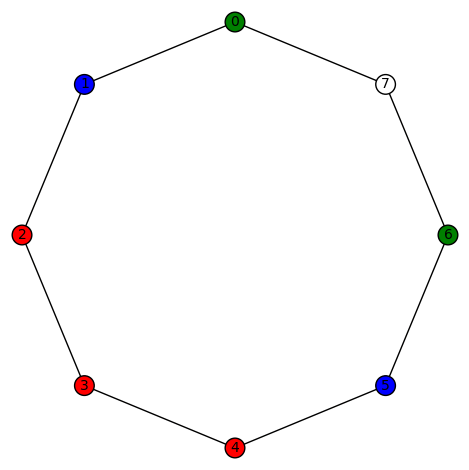
Example 5: There are 12 non-trivial harmonic morphisms 


or

by permutations of the vertices with a non-zero color (3!+3!=12).
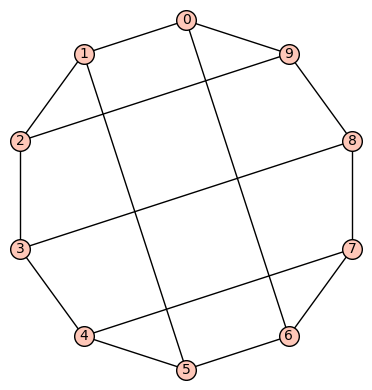
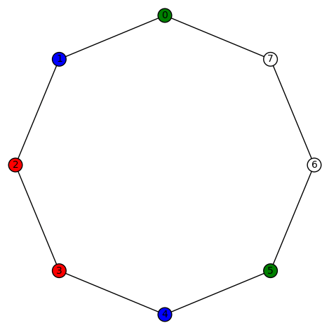
Example 6: There are 6 non-trivial harmonic morphisms 


by permutations of the vertices with a non-zero color (3!=6). This graph might be hard to visualize but it is isomorphic to the simple cubic graph having LCF notation [−4, 3, 3, 5, −3, −3, 4, 2, 5, −2]:

which has a nice picture. This is the ninth of the 19 simple cubic graphs on 10 vertices listed on this wikipedia page.
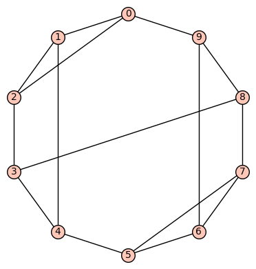
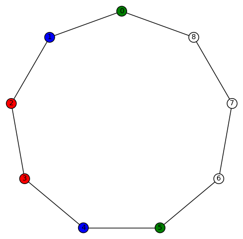
Example 7: (a) The first of the 19 simple cubic graphs on 10 vertices listed on this wikipedia page is the graph
This graph has diameter 5, automorphism group generated by (7,8), (6,9), (3,4), (2,5), (0,1)(2,6)(3,7)(4,8)(5,9). There are no non-trivial harmonic morphisms 
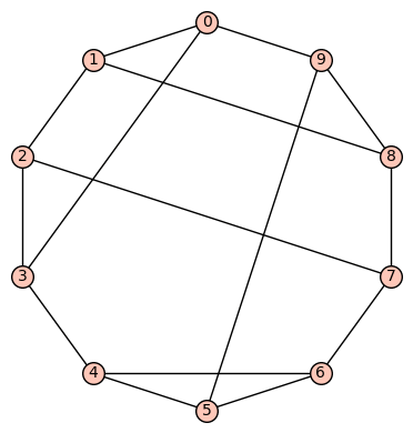
(b) The second of the 19 simple cubic graphs on 10 vertices listed on this wikipedia page is the graph

This graph has diameter 4, girth 3, automorphism group generated by (7,8), (0,5)(1,2)(6,9). There are no non-trivial harmonic morphisms
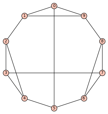
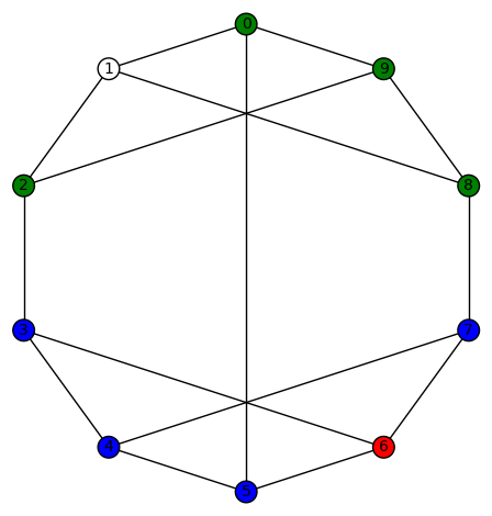
(c) The third of the 19 simple cubic graphs on 10 vertices listed on this wikipedia page is the graph

This graph has diameter 3, girth 3, automorphism group generated by (4,5), (0,1)(8,9), (0,8)(1,9)(2,7)(3,6). There are no non-trivial harmonic morphisms
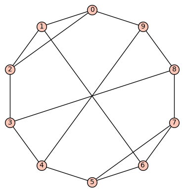
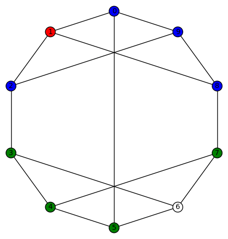
Example 8: The fourth of the 19 simple cubic graphs on 10 vertices listed on this wikipedia page is the graph

This graph has diameter 3, girth 3, automorphism group generated by (4,6), (3,5), (1,8)(2,7)(3,4)(5,6), (0,9). There are 12 non-trivial harmonic morphisms

and the remaining (3!=6 total) colorings obtained by permutating the non-zero colors. Another example is
and the remaining (3!=6 total) colorings obtained by permutating the non-zero colors.
Example 9: (a) The fifth of the 19 simple cubic graphs on 10 vertices listed on this wikipedia page is the graph
Its SageMath command is Gamma1 = graphs.LCFGraph(10,[2,2,-2,-2,5],2) There are no non-trivial harmonic morphisms
(b) The sixth of the 19 simple cubic graphs on 10 vertices listed on this wikipedia page is the graph
Its SageMath command is Gamma1 = graphs.LCFGraph(10,[2,3,-2,5,-3],2) There are no non-trivial harmonic morphisms
Example 10: The seventh of the 19 simple cubic graphs on 10 vertices listed on this wikipedia page is the graph

Its SageMath command is Gamma1 = graphs.LCFGraph(10,[2,3,-2,5,-3],2). Its automorphism group is order 12, generated by (1,2)(3,7)(4,6), (0,1)(5,6)(7,9), (0,4)(1,6)(2,5)(3,9). There are 6 non-trivial harmonic morphisms
Example 11: The eighth of the 19 simple cubic graphs on 10 vertices listed on this wikipedia page is the graph

Its SageMath command is Gamma1 = graphs.LCFGraph(10,[5, 3, 5, -4, -3, 5, 2, 5, -2, 4],1). Its automorphism group is order 2, generated by (0,3)(1,4)(2,5)(6,7). There are no non-trivial harmonic morphisms
Example 12: (a) The tenth (recall the 9th was mentioned above) of the 19 simple cubic graphs on 10 vertices listed on this wikipedia page is the graph
Its SageMath command is Gamma1 = graphs.LCFGraph(10,[3, -3, 5, -3, 2, 4, -2, 5, 3, -4],1). Its automorphism group is order 6, generated by (2,8)(3,9)(4,5), (0,2)(5,6)(7,9). There are no non-trivial harmonic morphisms
(b) The 11th of the 19 simple cubic graphs on 10 vertices listed on this wikipedia page is the graph

Its SageMath command is Gamma1 = graphs.LCFGraph(10,[-4, 4, 2, 5, -2],2). Its automorphism group is order 4, generated by (0,1)(2,9)(3,8)(4,7)(5,6), (0,5)(1,6)(2,7)(3,8)(4,9). There are no non-trivial harmonic morphisms
(c) The 12th of the 19 simple cubic graphs on 10 vertices listed on this wikipedia page is the graph
Its SageMath command is Gamma1 = graphs.LCFGraph(10,[5, -2, 2, 4, -2, 5, 2, -4, -2, 2],1). Its automorphism group is order 6, generated by (1,9)(2,8)(3,7)(4,6), (0,4,6)(1,3,8)(2,7,9). There are no non-trivial harmonic morphisms
(d) The 13th of the 19 simple cubic graphs on 10 vertices listed on this wikipedia page is the graph
Its SageMath command is Gamma1 = graphs.LCFGraph(10,[2, 5, -2, 5, 5],2). Its automorphism group is order 8, generated by (4,8)(5,7), (0,2)(3,9), (0,5)(1,6)(2,7)(3,8)(4,9). There are no non-trivial harmonic morphisms
Example 13: The 14th of the 19 simple cubic graphs on 10 vertices listed on this wikipedia page is the graph

By permuting the non-zero colors, we obtain 3!=6 harmonic morphisms from this one. Another harmonic morphism

By permuting the non-zero colors, we obtain 3!=6 harmonic morphisms from this one. And another harmonic morphism

By permuting the non-zero colors, we obtain 3!=6 harmonic morphisms from this one. Its SageMath command is Gamma1 = graphs.LCFGraph(10,[5, -3, -3, 3, 3],2). Its automorphism group is order 48, generated by (4,6), (2,8)(3,7), (1,9), (0,2)(3,5), (0,3)(1,4)(2,5)(6,9)(7,8). There are a total of 18=3!+3!+3! non-trivial harmonic morphisms
Example 14: The 15th of the 19 simple cubic graphs on 10 vertices listed on this wikipedia page is the graph

By permuting the non-zero colors, we obtain 3!=6 harmonic morphisms from this one. Its SageMath command is Gamma1 = graphs.LCFGraph(10,[5, -4, 4, -4, 4],2). Its automorphism group is order 8, generated by (2,7)(3,8), (1,9)(2,3)(4,6)(7,8), (0,5)(1,4)(2,3)(6,9)(7,8). There are a total of 6=3! non-trivial harmonic morphisms
Example 15: (a) The 16th of the 19 simple cubic graphs on 10 vertices listed on this wikipedia page is the graph

Its SageMath command is Gamma1 = graphs.LCFGraph(10,[5, -4, 4, 5, 5],2). Its automorphism group is order 4, generated by (0,3)(1,2)(4,9)(5,8)(6,7), (0,5)(1,6)(2,7)(3,8)(4,9). There are no non-trivial harmonic morphisms
(b) The 17th of the 19 simple cubic graphs on 10 vertices listed on this wikipedia page is the graph

Its SageMath command is Gamma1 = graphs.LCFGraph(10,[5, 5, -3, 5, 3],2). Its automorphism group is order 20, generated by (2,6)(3,7)(4,8)(5,9), (0,1)(2,5)(3,4)(6,9)(7,8), (0,2)(1,9)(3,5)(6,8). This group acts transitively on the vertices. There are no non-trivial harmonic morphisms
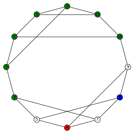
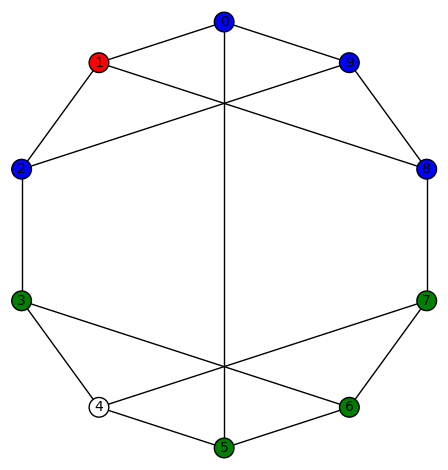
(c) The 18th of the 19 simple cubic graphs on 10 vertices listed on this wikipedia page is the graph
This is an example of a “thick polygon” graph, already mentioned in Example 3 above. Its SageMath command is Gamma1 = graphs.LCFGraph(10,[-4, 4, -3, 5, 3],2). Its automorphism group is order 20, generated by (2,5)(3,4)(6,9)(7,8), (0,1)(2,6)(3,7)(4,8)(5,9), (0,2)(1,9)(3,6)(4,7)(5,8). This group acts transitively on the vertices. There are no non-trivial harmonic morphisms
(d) The 19th in the list of 19 is the Petersen graph, already in Example 4 above.
We now consider some examples of the cubic graphs having 12 vertices. According to the House of Graphs there are 109 of these, but we use the list on this wikipedia page.
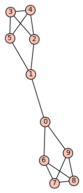
Example 16: I wrote a SageMath program that looked for harmonic morphisms on a case-by-case basis. If there is no harmonic morphism
, where
.
SageMath command:
V1 = [0,1,2,3,4,5,6,7,8,9,10,11]

E1 = [(0, 1), (0, 2), (0, 11), (1, 2), (1, 6), (2, 3), (3, 4), (3, 5), (4, 5), (4, 6), (5, 6), (7, 8), (7, 9), (7, 11), (8, 9), (8, 10), (9, 10), (10, 11)]

Gamma1 = Graph([V1,E1])
(Not in LCF notation since it doesn’t have a Hamiltonian cycle.)
.
SageMath command:
V1 = [0,1,2,3,4,5,6,7,8,9,10,11]

E1 = [(0, 1), (0, 6), (0, 11), (1, 2), (1, 3), (2, 3), (2, 5), (3, 4), (4, 5), (4, 6), (5, 6), (7, 8), (7, 9), (7, 11), (8, 9), (8, 10), (9, 10), (10, 11)]

Gamma1 = Graph([V1,E1])
(Not in LCF notation since it doesn’t have a Hamiltonian cycle.)
.
SageMath command:
V1 = [0,1,2,3,4,5,6,7,8,9,10,11]

E1 = [(0,1),(0,3),(0,11),(1,2),(1,6),(2,3),(2,5),(3,4),(4,5),(4,6),(5,6),(7,8),(7,9),(7,11),(8,9),(8,10),(9,10),(10,11)]

Gamma1 = Graph([V1,E1])
(Not in LCF notation since it doesn’t have a Hamiltonian cycle.)
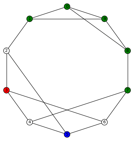
- This example has 12 non-trivial harmonic morphisms.
SageMath command:
V1 = [0,1,2,3,4,5,6,7,8,9,10,11]

E1 = [(0,1),(0,3),(0,11),(1,2),(1,6),(2,3),(2,5),(3,4),(4,5),(4,6),(5,6),(7,8),(7,9),(7,11),(8,9),(8,10),(9,10),(10,11)]

Gamma1 = Graph([V1,E1])
(Not in LCF notation since it doesn’t have a Hamiltonian cycle.) We show two such morphisms:

The other non-trivial harmonic morphisms are obtained by permuting the non-zero colors. There are 3!=6 for each graph above, so the total number of harmonic morphisms (including the trivial ones) is 6+6+4=16.
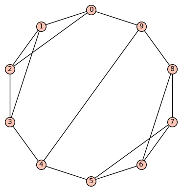
.
SageMath command:
Gamma1 = graphs.LCFGraph(12, [3, -2, -4, -3, 4, 2], 2)
- This example has 12 non-trivial harmonic morphisms.
. (This only differs by one edge from the one above.)
SageMath command:
Gamma1 = graphs.LCFGraph(12, [3, -2, -4, -3, 3, 3, 3, -3, -3, -3, 4, 2], 1)
We show two such morphisms:

And here is another plot of the last colored graph:
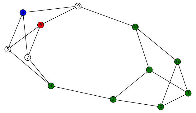
The other non-trivial harmonic morphisms are obtained by permuting the non-zero colors. There are 3!=6 for each graph above, so the total number of harmonic morphisms (including the trivial ones) is 6+6+4=16.
.
SageMath command:
Gamma1 = graphs.LCFGraph(12, [4, 2, 3, -2, -4, -3, 2, 3, -2, 2, -3, -2], 1)
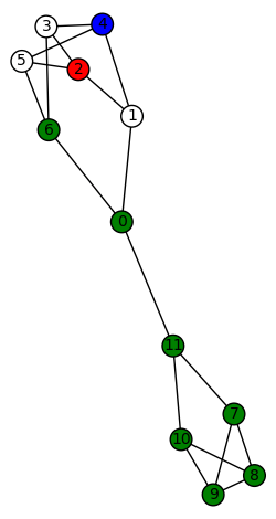
- This example has 48 non-trivial harmonic morphisms.
.
SageMath command:
Gamma1 = graphs.LCFGraph(12, [3, 3, 3, -3, -3, -3], 2)
This example is also interesting as it has a large number of automorphisms – its automorphism group is size 64, generated by (8,10), (7,9), (2,4), (1,3), (0,5)(1,2)(3,4)(6,11)(7,8)(9,10), (0,6)(1,7)(2,8)(3,9)(4,10)(5,11). Here are examples of some of the harmonic morphisms using vertex-colored graphs:


I think all the other non-trivial harmonic morphisms are obtained by (a) permuting the non-zero colors, or (b) applying a element of the automorphism group of the graph.
- (list under construction)
 .
.
 the white vertex is not adjacent to the blue or red vertex, none of the harmonic colored graphs below can have a white vertex adjacent to a blue or red vertex.
 as the domain in this post. However, before we get to examples (obtained by using
 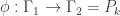 be a harmonic morphism from a graph
  vertices to the path graph having
  vertices. Let
  be the coloring map (identified with an n-tuple whose coordinates are in
  ). Associated to f is a partition
 ![\Pi_f=[n_0,\dots,n_{k-1}]](https://s0.wp.com/latex.php?latex=%5CPi_f%3D%5Bn_0%2C%5Cdots%2Cn_%7Bk-1%7D%5D&bg=ffffff&fg=323232&s=0&c=20201002) of n (here
of n (here ![[...]](https://s0.wp.com/latex.php?latex=%5B...%5D&bg=ffffff&fg=323232&s=0&c=20201002) is a multi-set, so repetition is allowed but the ordering is unimportant):
is a multi-set, so repetition is allowed but the ordering is unimportant):  , where
  is the number of times j occurs in f. We call this the partition invariant of the harmonic morphism.
  ,
,  , with associated
 whose corresponding partitions agree,
  then we say
  and
and  are partition equivalent.
 examples!
 , so we start with
  . We indicate a harmonic morphism by a vertex coloring. An example of a harmonic morphism can be described in the plot below as follows:
  sends the red vertices in
  , plus that induced by
  and all of its cyclic permutations (4+6=10). This set of 6 permutations is closed under the automorphism of
 and all of its cyclic permutations (4+7=11). This set of 7 permutations is not closed under the automorphism of
  and all 7 of its cyclic permutations (total = 7+11 = 18).

 and all of its cyclic permutations (4+8=12). This set of 8 permutations is not closed under the automorphism of
 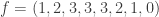 and all of its cyclic permutations (12+8=20). In addition, there is
  and all of its cyclic permutations (20+8 = 28). The latter set of 8 cyclic permutations of
  is closed under the transposition (0,3)(1,2) (total = 28).
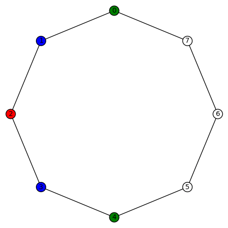
 and all of its cyclic permutations (4+9=13). This set of 9 permutations is not closed under the automorphism of
  and all 9 of its cyclic permutations (9+13 = 22). This set of 9 permutations is not closed under the automorphism of
  and all 9 of its cyclic permutations (9+22 = 31). This set of 9 permutations is not closed under the automorphism of
  and all 9 of its cyclic permutations (total = 9+31 = 40).


 is the graph whose SageMath command is
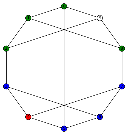


 then, instead of showing a graph, I’ll list the edges (of course, the vertices are 0,1,…,11) and the SageMath command for it.
 .
. .
.
 and
and  are graphs then a map
  ) is a morphism provided
 and
and  then
then  is an edge in
  and
and  , where
  then
then 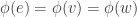 .
. is the dual map
  and
and  , then
  , an edge
  is called horizontal if
  and is called vertical if
  . We say that a graph morphism
  is a graph homomorphism if
  . Thus, a graph morphism is a homomorphism if it has no vertical edges.
 denote the star subgraph centered at the vertex v. A graph morphism
  is called harmonic if for all vertices
  , the quantity
 and mapping to the edge
  .
. sends the red vertices in

 such that two successive terms differ in only one position. A Gray code can be regarded as a Hamiltonian path in the cube graph. For example:
 denote the rating of Team
  ,
,  .
. denote an $n\times n$ matrix of score results:
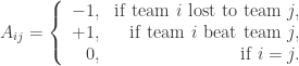
 .
. associated to the example of the Patriot league is the adjacency matrix of a diagraph.
 :
:  .
. , update their rating using the formula

 and
and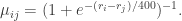

 Army
Army  .
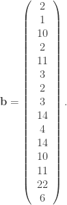
. , and the total runs allowed by team
  . Here, we order the six teams as above (team
  is Army (USMI at Westpoint), team
  is Bucknell, and so on). For instance if X played Y and the scores were
  ,
,  ,
,  in the position of row X and column Y.
 matrix:
 which best fits the equation

 with linearly independent columns. Unfortunately, in this case
  does not have linearly independent columns, so the formula doesn’t apply.
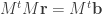


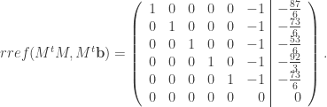
 denotes the rankings of Army, Bucknell, Holy Cross, Lafayette, Lehigh, Navy, in that order, then
 .
.
You must be logged in to post a comment.